How to find and highlight duplicate rows in a range in Excel?

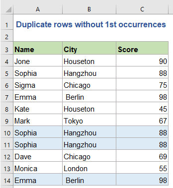
Sometimes, there are may be some duplicate records in your data range of a worksheet, and now you want to find or highlight the duplicate rows in the range as following screenshots shown. Of course you can find them one after one by checking for the rows. But this is not a good choice if there are hundreds of rows. Here, I will talk about some useful ways for you to deal with this task.


Find duplicate rows across multiple columns with formulas

Highlight duplicate rows across multiple columns with Conditional Formatting

Select or highlight duplicate rows across multiple columns with a handy feature


Find duplicate rows across multiple columns with formulas

The following formula can help you to find the duplicate records, please do as this:

1. In the adjacent blank cell, cell D2 in this case, please enter the below formula:

=IF(COUNTIFS($A$2:$A$12,$A2,$B$2:$B$12,$B2,$C$2:$C$12,$C2)>1, "Duplicate row", "")

2. And then drag the fill handle down to the cells for applying this formula, now, you can see, if there are identical rows in this used range, it will display Duplicate row, see screenshot:

  • Notes:
  • 1. In the formula, $A$2:$A$12, $B$2:$B$12, $C$2:$C$12 indicate the range columns that you want to find the duplicate from. You can change them as you want. And A2, B2, C2 indicate the first cells in the each column of the data which needed to be applied this formula, you can change them as well.
  • 2. The above formula is based on data in 3 columns, if there are 4 or more columns in your data range which needed to be found the duplicated values from the first row, you just need to add the column references as this formula shown: =IF(COUNTIFS($A$2:$A$12,$A2,$B$2:$B$12,$B2,$C$2:$C$12,$C2,$D$2:$D$12,$D2)>1, "Duplicate row", "").

Tips: If you want to find duplicate rows without the first occurrences, please apply the following formula:

=IF(COUNTIFS($A$2:$A2,$A2,$B$2:$B2,$B2,$C$2:$C2,$C2) >1, "Duplicate row", "")


Highlight duplicate rows across multiple columns with Conditional Formatting

If you can’t apply the formula correctly, please don’t worry, the Conditional Formatting utility also can help you to highlight the duplicate rows. Do with the following steps:

1. The first step you should to use the CONCATENATE function to combine all the data into one cell for each row. Type the below formulain cell D2, then copy the formula down until the last row of data see screenshot:
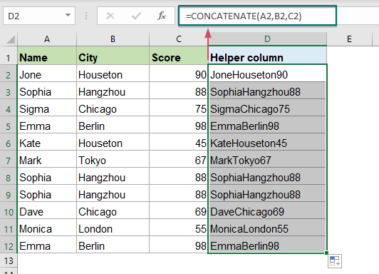
=CONCATENATE(A2,B2,C2)

2. Then, select the range that you want to find the duplicate rows including the formulas in column D, and then go to Home tab, and click Conditional Formatting > New Rule, see screenshot:

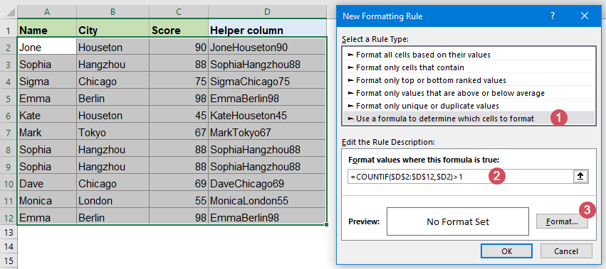
3. In the New Formatting Rule dialog box, please do the following operations:

  • Click Use a formula to determine which cells to format from the Select a Rule Type list box;
  • And then, enter this formula =COUNTIF($D$2:$D$12,$D2)>1 (Highlight duplicate rows with first occurrences) or =COUNTIF($D$2:$D2,$D2)>1 (Highlight duplicate rows without first occurrences) into the Format values where this formula is true text box;
  • At last, click Format button.

Note: In the above formula, $D$2:$D$12 is the column D that you have combined the other column values.

4. In the popped out Format Cells dialog box, click Fill tab, and then, choose one color that you need to highlight the duplicates.
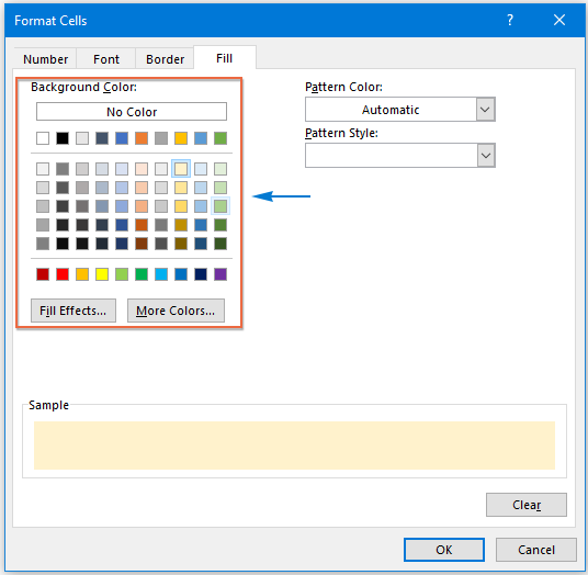
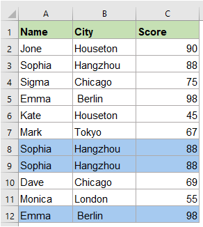
5. Click OK > OK to close the dialog boxes, and the duplicate rows are highlighted by the color you choose at once, see screenshot:

Highlight duplicate rows with the first ones Highlight duplicate row without the first ones

Select or highlight duplicate rows across multiple columns with a handy feature

The above methods are somewhat troublesome for you, so here, I can introduce you an easy and handy tool-Kutools for Excel, with its Select duplicate & unique cells utility, you can quickly select the duplicate rows or unique rows as you need.

Note:To apply this Select duplicate & unique cells, firstly, you should download the Kutools for Excel, and then apply the feature quickly and easily.

After installing Kutools for Excel, please do as this:

1. Click Kutools > Select > Select Duplicate & Unique Cells, see screenshot:

2. In the Select duplicate & unique cells dialog box, please do the following operations:

  • Click button1  button to select the range that you want to use;
  • Then, select Each row from the Based on section;
  • And then,check Duplicates(Except 1st one) or All duplicates(Including 1st one) option under Rule section as you need;
  • At last, you can specify a background color or font color for the duplicate rows under the Processing of results.
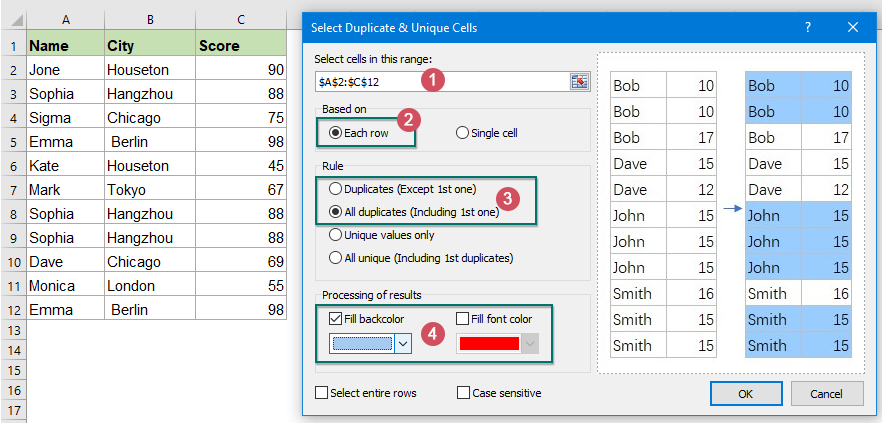
3. Then click OK, and the duplicate rows are selected as following screenshots:

Select duplicate rows including the first ones Select duplicate rows excluding the first ones
  • Notes:
  • 1. If you check Select entire rows option, the entire duplicate or unique rows will be selected.
  • 2. If you check Case sensitive option, the text will be compared case sensitive.

 Download and free trial Kutools for Excel Now !


More relative articles:

  • Combine Duplicate Rows And Sum The Values In Excel
  • In Excel,you may always meet this problem, when you have a range of data which contains some duplicate entries, and now you want to combine the duplicate data and sum the corresponding values in another column, as following screenshots shown. How could you solve this problem?
  • Highlight Duplicate Values In Different Colors In Excel
  • In Excel, we can easily highlight the duplicate values in a column with one color by using the Conditional Formatting, but, sometimes, we need to highlight the duplicate values in different colors to recognize the duplicates quickly and easily as following screenshot shown. How could you solve this task in Excel?
  • Align Duplicates Or Matching Values In Two Columns
  • If you have two list of names, and you want to compare these two columns and find the duplicates in both, and then align or display the matching names based on the first column in a new column as following screenshot shown. To list the duplicate values which exist in both columns, this article may introduce some tricks for solving it.

Best Office Productivity Tools

🤖 Kutools AI Aide: Revolutionize data analysis based on: Intelligent Execution   |  Generate Code  |  Create Custom Formulas  |  Analyze Data and Generate Charts  |  Invoke Kutools Functions
Popular Features: Find, Highlight or Identify Duplicates   |  Delete Blank Rows   |  Combine Columns or Cells without Losing Data   |   Round without Formula ...
Super Lookup: Multiple Criteria VLookup    Multiple Value VLookup  |   VLookup Across Multiple Sheets   |   Fuzzy Lookup ....
Advanced Drop-down List: Quickly Create Drop Down List   |  Dependent Drop Down List   |  Multi-select Drop Down List ....
Column Manager: Add a Specific Number of Columns  |  Move Columns  |  Toggle Visibility Status of Hidden Columns  |  Compare Ranges & Columns ...
Featured Features: Grid Focus   |  Design View   |   Big Formula Bar    Workbook & Sheet Manager   |  Resource Library (Auto Text)   |  Date Picker   |  Combine Worksheets   |  Encrypt/Decrypt Cells    Send Emails by List   |  Super Filter   |   Special Filter (filter bold/italic/strikethrough...) ...
Top 15 Toolsets12 Text Tools (Add Text, Remove Characters, ...)   |   50+ Chart Types (Gantt Chart, ...)   |   40+ Practical Formulas (Calculate age based on birthday, ...)   |   19 Insertion Tools (Insert QR Code, Insert Picture from Path, ...)   |   12 Conversion Tools (Numbers to Words, Currency Conversion, ...)   |   7 Merge & Split Tools (Advanced Combine Rows, Split Cells, ...)   |   ... and more

Supercharge Your Excel Skills with Kutools for Excel, and Experience Efficiency Like Never Before. Kutools for Excel Offers Over 300 Advanced Features to Boost Productivity and Save Time.  Click Here to Get The Feature You Need The Most...

Description


Office Tab Brings Tabbed interface to Office, and Make Your Work Much Easier

  • Enable tabbed editing and reading in Word, Excel, PowerPoint, Publisher, Access, Visio and Project.
  • Open and create multiple documents in new tabs of the same window, rather than in new windows.
  • Increases your productivity by 50%, and reduces hundreds of mouse clicks for you every day!
Comments (16)
No ratings yet. Be the first to rate!
This comment was minimized by the moderator on the site
Fórmulas lixo, nenhuma funciona!
This comment was minimized by the moderator on the site
Hello Carlos,
So sorry to hear that. But I did try all of the formulas in the article and they all works fine. Please see the screenshots I upload. And I would love to help you on this matter if only you could provide the details of the errors. Thanks.Sincerely,Mandy
This comment was minimized by the moderator on the site
The formula "Sumproduct" does not work! The values ​​keep appearing non-duplicate, and since there are duplicate values, you must have got something wrong with this formula. Because I did the same and checked several times to find the error, but I was unsuccessful
This comment was minimized by the moderator on the site
Hello, Elienay,
The above Sumproduct formula works well in my worksheet, could you give your problem as an image to insert here?
Thank you!
This comment was minimized by the moderator on the site
I had to invent another formula to check for duplicate values, in fact I created two formulas! But with this "sumproduct" I couldn't fix it. However I already solved my problem, thanks! The formula I created looked like this: =IF(CONTIF($G$53:$G$55;G53)>1;"DUPLI";"NO")
This comment was minimized by the moderator on the site
at the time of data entry can i stop duplicate entries in two columns example :- Table A Table B A 1 B 2 at the time data entry once A & 1 is coming than i don't enter this entry, can any formula & idea for this
This comment was minimized by the moderator on the site
Can i find duplicate entries in two columns at time of data entry, that can i prevent duplicate entries in two columns example, Table A Table B A 1 B 2 at time of data entry next A and 1 i don't enter this entry, plz give any idea
This comment was minimized by the moderator on the site
Hi, suppose i have data of 15 letters (alphanumeric), and i want it to be split in different columns. ex - ASDFGH11WE31005 this is the 15 letters code, i want it to be spilt in different columns like - AS DF GH 11 WE 3 1005 pls suggest any shortcut or any formula to split it
This comment was minimized by the moderator on the site
Good day, I am dealing with a similar problem but one that goes beyond just checking for duplicates and I am hoping you could shed some light in as to how to tackle it. To illustrate I will build up onto the problem you have already illustrated above and adding some more complexities to it. Suppose after checking for and finding duplicates (ie., product, order or quantity and price), you now want to select a shop from which you can now buy your products from (I assume the duplicates tells you what products in what amount you can buy at what prices, and there is that repeat of products, orders and prices). The Shop Name given is for the shop that actually has stock of items required. A B C D E F PRODUCT ORDER PRICE SHOP NAME Distance to Shop (miles) Shop chosen to buy from QQQQ 50 30 Shop A 15 ? PPPP 60 40 Shop A 15 ? XXXX 45 28 Shop B 30 ? QQQQ 50 30 Shop A 15 ? VVVV 65 42 Shop A 15 ? BBBB 48 21 Shop A 15 ? XXXX 45 28 Shop B 30 ? QQQQ 50 30 Shop B 30 ? MMMM 80 35 Shop B 30 ? Suppose you now know you can buy a product at the given quantities (order) and at the given prices, at either Shop A or Shop B or Shop B but now you want to decide on the shop to buy from. One of the factors used in the criteria for shop selection could be how far the shop is from your own location. Obviously for product XXXX the only shop to buy from, where the product is available is Shop B therefore the value to return under column E would always be Shop B. For product QQQQ, you would have the option of buying from either Shop A or Shop B. You now want Excel to have you choose a shop to buy from. You want to select the nearest shop. How would you go about using a formula to solve this one? Regards, Moses
This comment was minimized by the moderator on the site
Suppose you have now ascertained that there are duplicates and the next thing is you want to check is if these duplicates (products, orders, and prices) can be obtained are from different shops. This is tantamount to introducing another column listingshops which actaully sell these products and you want to be able to select a shop to buy from based on another criteria not listed here (knowledge of shop location,distance to the shop, etc) Eg for Product QQQ, you can get same order at same price at both Shop A and Shop B and you wanna return either Shop A or Shop B based on that criteria you know. How would you tell Excel to return as a value either either Shop A or Shop B? PRODUCT ORDER PRICE SHOP NAME QQQQ 50 30 Shop A PPPP 60 40 Shop A XXXX 45 28 Shop B QQQQ 50 30 Shop A VVVV 65 42 Shop A BBBB 48 21 Shop A XXXX 45 28 Shop B QQQQ 50 30 Shop B MMMM 80 35 Shop B
This comment was minimized by the moderator on the site
This is very very very great INFO !! i was so confused to find this kind of formula in excel sheet but today i am so happy may god give you lots of happiness and success, Great Work buddy you're a Champ !!
This comment was minimized by the moderator on the site
Great Great Great Really best ideas I've ever seen
This comment was minimized by the moderator on the site
Yes!!! NASEER you can find duplicates... :)
There are no comments posted here yet
Load More
Please leave your comments in English
Posting as Guest
×
Rate this post:
0   Characters
Suggested Locations