How to highlight rows when cell value changes in Excel?
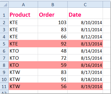
If there is a list of repeated values in your worksheet, and you need to highlight the rows based on column A which cell value changes as following screenshot shown. In fact, you can quickly and easily finish this job by using the Conditional Formatting feature.
Highlight rows when cell value changes with Conditional Formatting
 Highlight rows when cell value changes with Conditional Formatting

To highlight the rows which value is different from above value based on a column, you can apply a simple formula mixed with the Conditional Formatting.
1. Select your data range that you want to use, if your data has headers, exclude them.
2. Then click Home > Conditional Formatting > New Rule, see screenshot:

3. In the New Formatting Rule dialog, click Use a formula to determine which cells to format, and then enter this formula =$A3<>$A2 (A3, A2 in the column which you want to identify the cell value is different from the above value.)into the Format values where this formula is true text box, see screenshot:

4. And then click Format button to open the Format Cells dialog, under the Fill tab, choose one color you like, see screenshot:

5. Then click OK > OK to close the dialogs, and the rows have been highlighted which cell value changes based on column A.
Note: Conditional Formatting tool is a dynamic function, if you change values in column A or insert new row between the data, the formatting will be adjusted as well.
Tip: If your data has no headers, please enter this formula =$A2<>$A1 into the Format values where this formula is true text box
Related articles:
How to highlight / conditional formatting cells with formulas in Excel?
How to highlight all named ranges in Excel?
How to highlight cells based on length of text in Excel?
Best Office Productivity Tools
Supercharge Your Excel Skills with Kutools for Excel, and Experience Efficiency Like Never Before. Kutools for Excel Offers Over 300 Advanced Features to Boost Productivity and Save Time. Click Here to Get The Feature You Need The Most...
")
Office Tab Brings Tabbed interface to Office, and Make Your Work Much Easier
- Enable tabbed editing and reading in Word, Excel, PowerPoint, Publisher, Access, Visio and Project.
- Open and create multiple documents in new tabs of the same window, rather than in new windows.
- Increases your productivity by 50%, and reduces hundreds of mouse clicks for you every day!
")