How to auto update a chart after entering new data in Excel?
Suppose you have created a chart in Excel to visually track daily sales data, and you regularly update this data as new sales are recorded. Normally, whenever you insert or modify data in your range, you may need to manually adjust the chart’s data range to ensure the chart displays the most recent figures. This manual process can become repetitive and error-prone, especially with larger datasets or frequently changing information. Fortunately, there are practical methods to automatically update your charts when new data is added, helping keep your dashboard or reports consistently current.
There are several ways to achieve this automatic chart updating in Excel, each suited for different Excel versions and data layouts. The solutions explained below cover converting your data to an Excel table, using dynamic formulas with named ranges, and—especially useful for complex or custom requirements—applying a VBA macro.
Auto update a chart after entering new data with creating a table
Auto update a chart after entering new data with dynamic formula
Auto update a chart after entering new data with VBA code
 Auto update a chart after entering new data with creating a table
If you have a continuous range of data along with a corresponding column chart, you can ensure the chart updates instantly as you add new information by transforming the data range into an Excel table. This approach is available in Excel2007 and newer versions, and makes managing expanding datasets much easier. The main benefit is that charts referencing a table will automatically include new rows added to the table. Here is how you can do it:

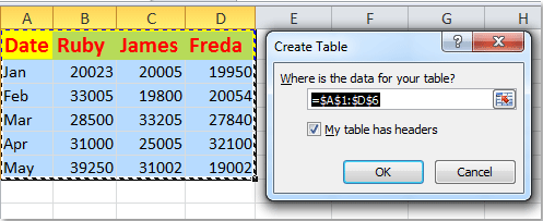
1. Select your existing data range that includes both headers and daily values. Then, go to the Insert tab and click Table. Please see the screenshot:

2. In the Create Table dialog box, ensure that the option My table has headers is checked if your data includes headers. Then click OK. (If your range does not contain headers, leave this box unchecked.)
3. Your selected data range will now be formatted as a structured Excel table. Notice the table style formatting is applied automatically, as shown below:

4. Now, whenever you add new rows directly beneath the last row of the table (such as entering data for June), both the table and linked chart will expand automatically, displaying the latest data without extra steps. See the example below for reference:

Notes and practical tips:
1. Newly entered data must be directly adjacent—meaning there should be no empty rows or columns separating new and existing data—or the table (and chart) will not recognize the extension.
2. You can insert new rows anywhere within the table; the chart will automatically update accordingly, which is useful for updating historical records as well.
3. If the chart is not updating as expected, check that the chart’s source data range is referencing the table, not a static range.

Unlock Excel Magic with Kutools AI
- Smart Execution: Perform cell operations, analyze data, and create charts—all driven by simple commands.
- Custom Formulas: Generate tailored formulas to streamline your workflows.
- VBA Coding: Write and implement VBA code effortlessly.
- Formula Interpretation: Understand complex formulas with ease.
- Text Translation: Break language barriers within your spreadsheets.
Auto update a chart after entering new data with dynamic formula
If you do not want to convert your data into an Excel table, you can use dynamic named ranges powered by formulas. This method leverages the OFFSET and COUNTA functions to define ranges that automatically resize according to the actual amount of data present. This approach is particularly useful when your data structure is fixed, but entries may be added or removed regularly. See the practical steps below:

1. Begin by defining a dynamic named range for each data column. Go to the Formulas tab and click Define Name.
2. In the New Name dialog, enter an appropriate name (e.g., Date for the date column), select the correct worksheet under Scope, and enter the dynamic formula into the Refers to field. For instance: =OFFSET($A$2,0,0,COUNTA($A:$A)-1). Refer to the screenshot for reference:

3. Click OK to save. Repeat the steps for each relevant series or data column, using formulas such as:
- Column B: Ruby: =OFFSET($B$2,0,0,COUNTA($B:$B)-1);
- Column C: James: =OFFSET($C$2,0,0,COUNTA($C:$C)-1);
- Column D: Freda: =OFFSET($D$2,0,0,COUNTA($D:$D)-1)
These dynamic named ranges ensure that as new data is added to each column, the range expands or contracts automatically. Be aware that the OFFSET formula begins from your first data row, while COUNTA adapts the range size according to the total number of non-empty cells in the specified column.
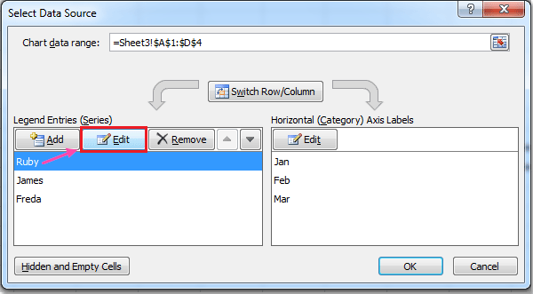
4. After defining all named ranges, right-click one of the columns in the linked chart and select Select Data from the context menu.

5. In the Select Data Source dialog box, highlight the relevant series (e.g., Ruby), click Edit, and enter the appropriate dynamic range as the Series values (for example, =Sheet3!Ruby). See below:
 |
 |
6. Repeat for each additional series, referencing the corresponding dynamic named range:
- James: Series values: =Sheet3!James;
- Freda: Series values: =Sheet3!Freda
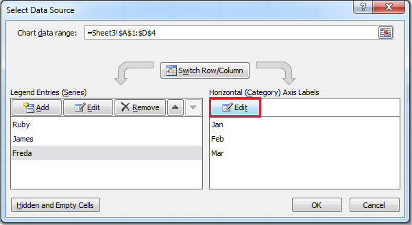
7. For the horizontal (category) axis labels, click Edit under Horizontal (Category) Axis Labels and supply the dynamic range name for the date column.
 |
 |
8. Click OK to confirm and exit all dialogs. From now on, as you continue to add new data entries in your worksheet, the chart will update itself automatically to reflect the latest data points.

- 1. Data must be typed into contiguous cells in the columns—the dynamic formula does not account for gaps between rows. If you skip rows, automatic extension may not function as intended.
- 2. This approach does not pick up additional series or columns if new headers are added; you’ll need to create new named ranges and update the chart data source accordingly.
- 3. If a dynamic range doesn’t expand, double-check the COUNTA range and ensure no extraneous entries exist below your intended data.
- 4. If you change worksheet names or cell locations, update the named range references to maintain dynamic behavior.
Auto update a chart after entering new data with VBA code
For advanced requirements—such as handling non-contiguous data, automatically detecting entirely new data series, or updating multiple charts simultaneously—a VBA macro can provide greater flexibility and automation. By writing a short macro that responds to data changes, you can automate the process of refreshing a chart's data source, responding to more complex scenarios that the previous methods cannot cover directly.
This solution is recommended if your data is spread out or not in a regular block, or when you routinely add new series or columns to your chart. Please follow the steps below to set this up:
1. Firstly, insert your chart as normal.
2. Press Alt + F11 to open the VBA editor.
3. In the VBA editor, click Insert > Module to insert a new code module. Then, enter the following macro code into the module window:
Sub AutoUpdateChartData()
    Dim ws As Worksheet
    Dim chrt As ChartObject
    Dim lastRow As Long

    On Error Resume Next
    xTitleId = "KutoolsforExcel"

    Set ws = ActiveSheet
    Set chrt = ws.ChartObjects(1) ' Modify if you have more than 1 chart on the sheet

    ' Find the last row of data in column A (assume your data starts from A1, adjust as needed)
    lastRow = ws.Cells(ws.Rows.Count, "A").End(xlUp).Row

    ' Set the data range for the chart dynamically (Modify range as per your data location)
    chrt.Chart.SetSourceData Source:=ws.Range("A1:D" & lastRow)

    On Error GoTo 0
End Sub3. To run the macro, click Run button. Your chart will now instantly update to reflect all current data up to the last populated row.
For enhanced automation, you can set this macro to trigger automatically whenever new data is entered.
To apply this, right-click your worksheet tab, select View Code, and paste the above code into the worksheet module. The macro will now run whenever you make changes to the sheet, ensuring the chart always stays up to date.
Private Sub Worksheet_Change(ByVal Target As Range)
    On Error Resume Next
    xTitleId = "KutoolsforExcel"
    Call AutoUpdateChartData
End Sub
Tips and notes:
- Your data range (e.g., "A1:D" & lastRow) should be modified to match the actual location and structure of your dataset. For non-contiguous ranges, consider customizing the range string directly in the code.
- If there are multiple charts, you may need to adjust ChartObjects(1) to reference the correct chart, or loop through all ChartObjects on the worksheet as needed.
- This VBA solution provides maximum flexibility for dynamic and complex datasets, but requires enabling macros and saving the file as a macro-enabled workbook (.xlsm).
- If the chart does not update as expected, double-check that the source data range in the macro matches your actual data block, and ensure macros are enabled in your Excel environment.
Related articles:
How to add a horizontal average line to chart in Excel?
How to create combination charts and add secondary axis for it in Excel?
Best Office Productivity Tools
Supercharge Your Excel Skills with Kutools for Excel, and Experience Efficiency Like Never Before. Kutools for Excel Offers Over 300 Advanced Features to Boost Productivity and Save Time. Click Here to Get The Feature You Need The Most...
Office Tab Brings Tabbed interface to Office, and Make Your Work Much Easier
- Enable tabbed editing and reading in Word, Excel, PowerPoint, Publisher, Access, Visio and Project.
- Open and create multiple documents in new tabs of the same window, rather than in new windows.
- Increases your productivity by 50%, and reduces hundreds of mouse clicks for you every day!
All Kutools add-ins. One installer
Kutools for Office suite bundles add-ins for Excel, Word, Outlook & PowerPoint plus Office Tab Pro, which is ideal for teams working across Office apps.
- All-in-one suite — Excel, Word, Outlook & PowerPoint add-ins + Office Tab Pro
- One installer, one license — set up in minutes (MSI-ready)
- Works better together — streamlined productivity across Office apps
- 30-day full-featured trial — no registration, no credit card
- Best value — save vs buying individual add-in