How to add color to drop down list in Excel?
In Excel, create a drop-down list can help you a lot, and sometimes, you need to color coded the drop down list values depending on the corresponding selected. For instance, I have created a drop-down list of the fruit names, when I select Apple, I need the cell is colored with red automatically, and when I choose Orange, the cell can be colored with orange as following screenshot shown. Are there any good suggestions to solve this?
Method A Color coded drop down list with Conditional Formatting
Method B Color coded drop down list with a handy tool-Colored Drop-down List
For finishing this task, we need to create a drop down list first, please do as following steps:
First, create a drop-down list:
1. Create a list of data and select a range that you want to put the drop down list values into. In this case, I select range A2:A6 to put the drop-down list, see screenshot:

2. Click Data > Data Validation > Data Validation, see screenshot:

3. And in the Data Validation dialog box, click Settings tab, and choose List option from the Allow drop down list, and then click to select the list values that you want to use. See screenshot:

4. Then click OK, the drop-down list has been created as following shown:

Now, you can add color to drop-down list, choose one method as you need.
1. Highlight your drop-down cells (here is column A), and go to click Home > Conditional Formatting > New Rule, see screenshot:

2. In the New Formatting Rule dialog box, click Format only cells that contain option in the Select a Rule Type section, under the Format only cells with section, choose Specific Text from the first drop down list and select containing from the second drop down, then click ![]() button to select the value that you want to format a specific color, see screenshot:
button to select the value that you want to format a specific color, see screenshot:

3. Then click Format button, and select one color you like from the Fill tab.

4. And then click OK > OK to close the dialogs, repeat steps 5 to 7 for each other drop down selection, for example, Peach for pink, Grape for purple…

5. After setting the colors for the values, when you choose anyone value from the drop-down menu, the cell will be colored with its specified color automatically.

If you want to handle this job more quickly, you can try the Colored Drop-down List tools of Kutools for Excel, which can help you directly add colors to the items of drop-down list.
After free installing Kutools for Excel, please do as below:
1. Select the drop-down list cells, then click Kutools > Drop-down List > Colored Drop-down List.
2. In the Colored Drop-down list dialog, do below settings.
1) Check the scale you want to add color to in the Apply to section.

If you check Row of data range in the Apply to section, you need to select the row range.

2) Add colors to the items of drop-down list one by one.
Click at one item in the List Items, then click one color you need to add the color to the selected item.

Repeat the step to add colors to all items.
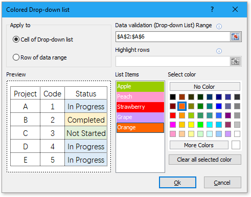
3. Click Ok. Now the items in drop-down list have been colored.

Autocomplete when typing in Excel drop down list
If you have a data validation drop down list with large values, you need to scroll down in the list just for finding the proper one, or type the whole word into the list box directly. If there is method for allowing to auto complete when typing the first letter in the drop down list, everything will become easier.
Create a dependent drop down list in Google sheet
Inserting normal drop down list in Google sheet may be an easy job for you, but, sometimes, you may need to insert a dependent drop down list which means the second drop down list depending on the choice of the first drop down list.
Create a drop down list from another drop down list in Excel
In this tutorial, I introduce the way to create a drop down list from another drop down list as below screenshot shown in Excel.
Create a dynamic drop down list in alphabetical order in Excel
Most of you may know how to create a dynamic drop down list, but in some cases, you may want to sort the drop down list in alphabetical order as below screenshot shown. Now this tutorial introduces the way to create a dynamic drop down list in alphabetical order in Excel
Best Office Productivity Tools
Supercharge Your Excel Skills with Kutools for Excel, and Experience Efficiency Like Never Before. Kutools for Excel Offers Over 300 Advanced Features to Boost Productivity and Save Time. Click Here to Get The Feature You Need The Most...
Office Tab Brings Tabbed interface to Office, and Make Your Work Much Easier
- Enable tabbed editing and reading in Word, Excel, PowerPoint, Publisher, Access, Visio and Project.
- Open and create multiple documents in new tabs of the same window, rather than in new windows.
- Increases your productivity by 50%, and reduces hundreds of mouse clicks for you every day!