Auto-highlight active row and column in Excel (Full Guide)
Navigating through extensive Excel worksheets brimming with data can be challenging, and it's easy to lose track of your place or misread values. To enhance your data analysis and reduce the chance of errors, we will introduce 3 different ways to dynamically highlight the row and column of a selected cell in Excel. As you move from cell to cell, the highlighting dynamically shifts, providing a clear and intuitive visual cue to keep you focused on the correct data as following demo shown:
Auto-highlight active row and column in Excel
- With VBA code-Clears the existing cell color, does not support Undo
- Only one click of Kutools for Excel -Keeps existing cell color, supports Undo, applies in protected sheets
- With Conditional Formatting -Not stable in large data, requires manual refresh (F9)
Auto-highlight active row and column with VBA code
To automatically highlight the entire column and row of the selected cell in current worksheet, the following VBA code may help you to achieve this task.
Step 1: Open the worksheet where you want to auto-highlight active row and column
Step 2: Open the VBA sheet module editor and copy the code
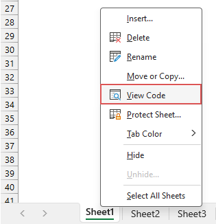
- Right click the sheet name, and choose "View Code" from the context menu, see screenshot:

- In the opened VBA sheet module editor, copy and paste the following code into the blank module. See screenshot:
VBA code: auto-highlight row and column of selected cellPrivate Sub Worksheet_SelectionChange(ByVal Target As Range) 'Update by Extendoffice Dim rowRange As Range Dim colRange As Range Dim activeCell As Range Set activeCell = Target.Cells(1, 1) Set rowRange = Rows(activeCell.Row) Set colRange = Columns(activeCell.Column) Cells.Interior.ColorIndex = xlNone rowRange.Interior.Color = RGB(248, 150, 171) colRange.Interior.Color = RGB(173, 233, 249) End SubTips: Customize the code- To change the highlight color, you simply need to modify the RGB value in the following scripts:
rowRange.Interior.Color = RGB(248, 150, 171)
colRange.Interior.Color = RGB(173, 233, 249) - To only highlight the entire row of selected cell, remove or comment out (add an apostrophe at the front of) this line:
colRange.Interior.Color = RGB(173, 233, 249) - To only highlight the entire column of selected cell, remove or comment out (add an apostrophe at the front of) this line:
rowRange.Interior.Color = RGB(248, 150, 171)

- To change the highlight color, you simply need to modify the RGB value in the following scripts:
- Then, close the VBA editor window to return to the worksheet.
Result:
Now, when you select a cell, the entire row and column of that cell are automatically highlighted, and the highlight dynamically shifts as the selected cell changes as below demo shown:
- This code will clear the background colors from all cells in the worksheet, so, avoid using this solution if you have cells with custom coloring.
- Running this code will disable the "Undo" feature in the sheet, meaning you cannot reverse any mistakes by pressing the "Ctrl" + "Z" shortcut.
- This code will not work in a protected worksheet.
- To stop highlighting the row and column of the selected cell, you'll need to remove the previously added VBA code. After that, to reset the highlighting by clicking "Home" > "Fill color" > "No fill".
Auto-highlight active row and column with only one click of Kutools
Facing the limitations of VBA code in Excel? The "Grid Focus" feature of "Kutools for Excel" is your ideal solution! Designed to address the shortcomings of VBA, it offers a diverse array of highlighting styles to enhance your sheet experience. With its ability to apply these styles across all open workbooks, "Kutools" ensures a consistently efficient and visually appealing data management process.
After installing Kutools for Excel, please click "Kutools" > "Grid Focus" to enable this feature. Now, you can see the row and column of active cell are highlighted immediately. This highlight dynamically shifts to follow as you change your cell selection. See the demo below:
- Preserves original cell background colors:
Unlike the VBA code, this feature respects your worksheet’s existing formatting. - Usable in protected sheets:
This feature works seamlessly within protected worksheets, making it ideal for managing sensitive or shared documents without compromising security. - Does not impact the Undo function:
With this feature, you retain full access to Excel's undo functionality. This ensures that you can easily revert changes, adding a layer of safety to your data manipulation. - Stable performance with large data:
This feature is designed to handle large datasets efficiently, ensuring stable performance even in complex and data-intensive spreadsheets. - Multiple highlighting styles:
This feature offers a variety of highlighting options, allowing you to choose from different styles and colors to make your active cell of row, column or row and column stand out in a way that best suits your preferences and needs.
- To disable this feature, please click "Kutools" > "Grid Focus" again to close this function;
- To apply this feature, please download and install Kutools for Excel.
Auto-highlight active row and column with Conditional Formatting
In Excel, you can also set up Conditional Formatting to auto-highlight the active row and column. For setting up this feature, please follow these steps:
Step 1: Select the data range
First, select the range of cells you want this feature to apply to. This could be the entire worksheet or a specific data set. Here, I will select the whole worksheet.
Step 2: Access Conditional Formatting
Click "Home" > "Conditional Formatting" > "New Rule", see screenshot:
Step 3: Set the operations in the New Formatting Rule
- In the "New Formatting Rule" dialog box, choose "Use a formula to determine which cells to format" from the "Select a Rule Type" list box.
- In the "Format values where this formula is true" box, enter one of these formulas, in this example, I will apply the third formula to highlight the active row and column.
To highlight active row:
To highlight active column:=CELL("row")=ROW()
To highlight active row and column:=CELL("col")=COLUMN()=OR(CELL("row")=ROW(), CELL("col")= COLUMN()) - Then, click "Format" button.

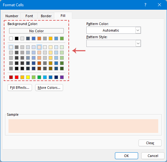
- In the following "Format Cells" dialog box, under the "Fill" tab, choose one color to highlight the active row and column as you need, see screenshot:

- Then, click "OK" > "OK" to close the dialogs.
Result:
Now, you can see the whole column and row of cell A1 have been highlighted at once. To apply this highlighting to another cell, simply click on your desired cell and press the "F9" key to refresh the sheet, which will then highlight the entire column and row of the newly selected cell.
- Indeed, while the Conditional Formatting approach for highlighting in Excel offers a solution, it's not as seamless as using "VBA" and "Grid Focus" feature. This method necessitates manual recalculation of the sheet (achieved by pressing the "F9" key).
To enable automatic recalculation of your worksheet, you can incorporate a simple VBA code into the code module of your target sheet. This will automate the refresh process, ensuring the highlighting updates immediately as you select different cells without pressing the "F9" key. Please right click the sheet name, and then choose "View Code" from the context menu. Then copy and paste the following code into the sheet module:Private Sub Worksheet_SelectionChange(ByVal Target As Range) Target.Calculate End Sub - The Conditional Formatting preserves the existing formatting you have manually applied to your worksheet.
- Conditional Formatting is known to be volatile, especially when applied to very large datasets. Its extensive use can potentially slow down your workbook's performance, affecting the efficiency of data processing and navigation.
- The CELL function is only available in Excel versions 2007 and later, this method is not compatible with earlier versions of Excel.
Comparison of the above Methods
| Feature | VBA code | Conditional Formatting | Kutools for Excel |
| Preserve cell background color | No | Yes | Yes |
| Supports Undo | No | Yes | Yes |
| Stable in large datasets | No | No | Yes |
| Usable in protected sheets | No | Yes | Yes |
| Applies to all open workbooks | Only current sheet | Only current sheet | All open workbooks |
| Requires manual refresh (F9) | No | Yes | No |
That concludes our guide on how to highlight the column and row of a selected cell in Excel. If you're interested in exploring more Excel tips and tricks, our website offers thousands of tutorials, please click here to access them. Thank you for reading, and we look forward to providing you with more helpful information in the future!
Related Articles:
- Auto-highlight row and column of active cell
- When you view a large worksheet with numerous data, you may want to highlight the selected cell’ row and column so that you can easily and intuitively read the data to avoid misreading them. Here, I can introduce you some interesting tricks to highlight the row and column of the current cell, when the cell is changed, the column and row of the new cell are highlighted automatically.
- Highlight every other row or column in Excel
- In a large worksheet, highlighting or filling every other or every nth row or column improves data visibility and readability. It not only makes the worksheet look neater but also helps you understand the data faster. In this article, we'll guide you through various methods to shade every other or nth row or column, helping you present your data in a more appealing and straightforward manner.
- Highlight entire / whole row while scrolling
- If you have a large worksheet with multiple columns, it will be difficult for you to distinguish data on that row. In this case, you can highlight the whole row of active cell so that you can quickly and easily view the data in that row when you scroll down the horizontal scroll bar .This article, I will talk about some tricks for you to solve this problem.
- Highlight rows based on drop down list
- This article will talk about how to highlight rows based on drop down list, take the following screenshot for example, when I select “In Progress” from the drop down list in column E, I need to highlight this row with red color, when I select “Completed” from the drop down list, I need to highlight this row with blue color, and when I select “Not Started”, a green color will be used to highlight the row.
Best Office Productivity Tools
Supercharge Your Excel Skills with Kutools for Excel, and Experience Efficiency Like Never Before. Kutools for Excel Offers Over 300 Advanced Features to Boost Productivity and Save Time. Click Here to Get The Feature You Need The Most...
Office Tab Brings Tabbed interface to Office, and Make Your Work Much Easier
- Enable tabbed editing and reading in Word, Excel, PowerPoint, Publisher, Access, Visio and Project.
- Open and create multiple documents in new tabs of the same window, rather than in new windows.
- Increases your productivity by 50%, and reduces hundreds of mouse clicks for you every day!
All Kutools add-ins. One installer
Kutools for Office suite bundles add-ins for Excel, Word, Outlook & PowerPoint plus Office Tab Pro, which is ideal for teams working across Office apps.
- All-in-one suite — Excel, Word, Outlook & PowerPoint add-ins + Office Tab Pro
- One installer, one license — set up in minutes (MSI-ready)
- Works better together — streamlined productivity across Office apps
- 30-day full-featured trial — no registration, no credit card
- Best value — save vs buying individual add-in


