How to extract unique values from multiple columns in Excel?

If you often work with datasets spread across several columns in Excel, you may face situations where certain values are duplicated within the same column or between different columns. In many reporting or data analysis tasks, it becomes necessary to identify and extract all unique values—those that appear only once across the whole selection, regardless of where they are located. Doing this manually can be time-consuming and error-prone, especially when dealing with large datasets or complex tables. Fortunately, Excel offers a range of methods to efficiently extract these unique values.

This guide introduces several solutions you can use based on your Excel version and your preferences—such as formulas suitable for all versions, dynamic array formulas for recent versions, the use of Kutools AI Aide for straightforward results, Pivot Tables for visual consolidation, and VBA code for automated extraction in complex scenarios.

• Extract unique values from multiple columns with formulas
  • Array formula (all Excel versions)
  • Formula (Excel 365, Excel 2021, and newer versions)
• Extract unique values from multiple columns with Kutools AI Aide
• Extract unique values from multiple columns with Pivot Table
• Extract unique values from multiple columns with VBA code

Extract unique values from multiple columns with formulas

There are times when you would like to achieve this extraction with built-in Excel functions. This section details how to do so using two approaches: an array formula suitable for all versions of Excel, and a dynamic array formula available in newer versions like Excel 365 and Excel 2021. These methods are ideal when you want a direct formula-based solution, require frequent updating as your data changes, or need to avoid external add-ins or code.

Extract unique values from multiple columns with Array formula for all Excel versions

For compatibility across all Excel versions, using an array formula lets you extract unique values from several columns—even if your Excel does not support dynamic arrays. This approach utilizes a combination of INDIRECT, TEXT, MIN, IF, COUNTIF, ROW, and COLUMN functions, making it flexible for various data structures.

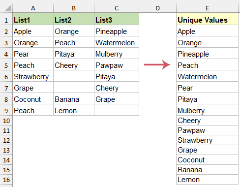
Suppose your data is located in the range A2:C9. To extract the unique values starting in cell E2, use the following procedure:

1. Click cell E2 (or the first cell of your output range), and input the following array formula:

=INDIRECT(TEXT(MIN(IF(($A$2:$C$9<>"")*(COUNTIF($E$1:E1,$A$2:$C$9)=0),ROW($2:$9)*100+COLUMN($A:$C),7^8)),"R0C00"),)&""

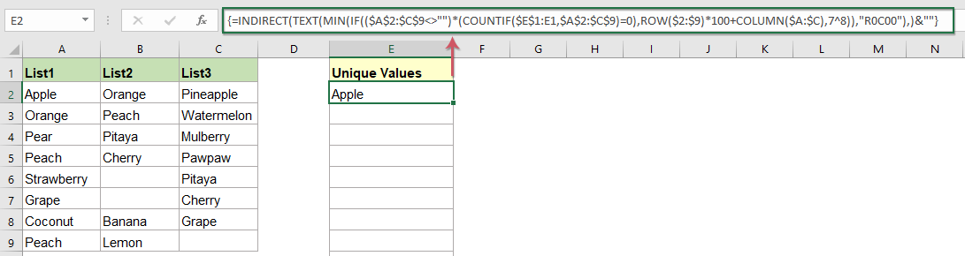
2. Once you have entered the formula, instead of just pressing Enter, press Ctrl + Shift + Enter together to confirm it as an array formula. When done correctly, curly brackets {} will appear around your formula in the formula bar. Then, drag the fill handle from E2 down the column. Continue dragging until blank cells appear, indicating there are no more unique values left to extract. This process ensures all unique values will be displayed in the target column.

Extract unique values from multiple columns with formula for Excel 365, Excel 2021, and newer versions

If you use Excel 365, Excel 2021, or a newer version, you have access to dynamic array functions, which provide a simpler and more intuitive way to extract unique values from multiple columns. The UNIQUE and TOCOL functions make it easier and faster to combine data across columns and eliminate duplicates in a single step—especially useful for those working with constantly updating or larger datasets.

To use this method, simply select a blank cell (for example, E2, or wherever you'd like the results to appear), enter this formula, and press Enter:

=UNIQUE(TOCOL(A2:C9,1))

After pressing Enter, all unique values from the range A2:C9 will spill into the cells below the formula automatically. This feature is particularly efficient—the output updates dynamically as your source data changes, saving you manual refresh steps.

Extract unique values from multiple columns with Kutools AI Aide

If you’d like a more streamlined approach and want to reduce manual effort, Kutools AI Aide in Kutools for Excel can help you extract unique values from multiple columns with ease. This method is especially valuable if you aren’t familiar with formulas or want to avoid the risk of formula errors. Kutools AI Aide interprets your instructions and processes the data automatically, which is ideal for both beginners and users looking for a quick solution in just a few clicks.

After installation, click Kutools AI > AI Aide to open the "Kutools AI Aide" pane:

1. Enter your request in the chat box, such as: "Extract unique values from the range A2:C9, ignoring blank cells, and place the results starting at E2:"
2. Click "Send" or press Enter, then after AI analyzes the request, simply click "Execute" to run. The results will instantly appear in your worksheet, at the exact location you indicated.

Tip: This solution is very useful if your data extraction workflow varies or if you want natural language processing features. Remember to double-check the extracted list for blank cells if your original data is not perfectly consistent, as blank entries might be included or filtered based on your AI request details.

Extract unique values from multiple columns with Pivot Table

Pivot Tables are another convenient method for extracting unique values, particularly if you prefer working with visual tools and want to summarize or further analyze the unique items, such as counting occurrences. This approach is straightforward and doesn't require formulas. However, it requires a few steps of setup and slight data rearrangement, especially if the columns involved have different headings.

Here is a suggested process for extracting unique values using a Pivot Table:

1. Insert a new blank column immediately to the left of your data. For example, insert a new column A if your data starts at column B. This adjustment helps ensure correct range consolidation.

2. Select any cell within your dataset, press Alt + D, then quickly press P to launch the "PivotTable and PivotChart Wizard." In the wizard's first step, select "Multiple consolidation ranges." This allows you to combine values from numerous columns into a single summarized field.

3. Click Next, then choose "Create a single page field for me." This step organizes all your data as a single group for easier unique value extraction.

4. In the next step, select the entire data range (include the new blank column), click the Add button to bring your selection into the "All ranges" list, and click Next.

5. In the wizard's final step, select where you would like to place the Pivot Table (new worksheet or existing sheet), then click Finish to generate the Pivot Table report.

6. In the new Pivot Table, uncheck all fields in the "Choose fields to add to report" section to clear the default view.

7. Finally, drag the "Value" field to the Rows area. The Pivot Table will display all unique values from your original multi-column range, organized neatly in a single column.

Extract unique values from multiple columns with VBA code

In cases where you need to automate extraction or handle large and irregular datasets, using VBA (Visual Basic for Applications) code can provide a quick and reusable solution. This is ideal for users with basic familiarity with the Excel VBA editor, or for recurring tasks where you want to minimize manual operations. VBA can also handle large data volumes more efficiently than array formulas.

1. Open the VBA editor by pressing Alt + F11. In the "Microsoft Visual Basic for Applications" window that appears, click Insert > Module to add a new module.

2. In the new module, paste the code below:

VBA: Extract unique values from multiple columns

Sub Uniquedata()
'Updateby Extendoffice
Dim rng As Range
Dim InputRng As Range, OutRng As Range
Set dt = CreateObject("Scripting.Dictionary")
xTitleId = "KutoolsforExcel"
Set InputRng = Application.Selection
Set InputRng = Application.InputBox("Range :", xTitleId, InputRng.Address, Type:=8)
Set OutRng = Application.InputBox("Out put to (single cell):", xTitleId, Type:=8)
For Each rng In InputRng
    If rng.Value <> "" Then
        dt(rng.Value) = ""
    End If
Next
OutRng.Range("A1").Resize(dt.Count) = Application.WorksheetFunction.Transpose(dt.Keys)
End Sub

3. Press F5 to run the code. A dialog will prompt you to select the data range. Select all relevant columns (including any with blank cells).

4. After clicking OK, another prompt asks where to output the unique values. Specify a top cell where you want the results listed (e.g., E2).

5. Click OK, and the macro will run automatically. All unique values will appear, starting at your specified location.

More relative articles: