How to create drop down list with images in Excel?
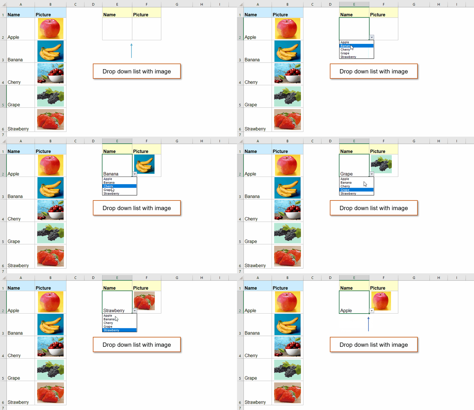
In Excel, we can quickly and easily create a drop down list with cell values, but, have you ever tried to create a drop down list with images, that is to say, when you click one value from the drop down list, its relative image will be displayed at once as below demo shown. In this article, I will talk about how to insert a drop down list with images in Excel.

Create a drop down list with image by Named Range feature
Create multiple drop down lists with images by a powerful feature
Insert multiple pictures based on cell values with a useful feature
Create a drop down list with image by Named Range feature
Normally, you can create a named range, and then use the linked picture for solving this task in Excel.
1. First, you should create two columns which contain the cell values and their relative images, see screenshot:

2. Then, you need to create a drop down list with the cell values, please click one cell where you want to output the drop down list value, and then click Data > Data Validation > Data Validation, see screenshot:

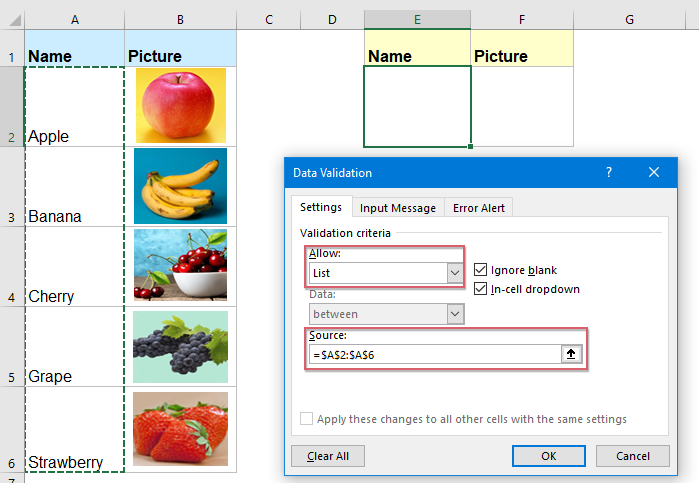
3. In the Data Validation dialog box, under the Settings tab, choose List from the Allow drop down list, and then select the cell values that you want to create the drop down list under Source section, see screenshot:

4. Then click OK button, and the drop down list with the cell values has been created, select one item from the drop down list, see screenshot:

5. Then, click Formulas > Define Name, see screenshot:

6. In the New Name dialog box, please do the following operations:
- Enter a name called myimage into the Name text box;
- Then copy and paste this formula: =INDEX(Sheet1!$A$2:$B$6,MATCH(Sheet1!$E$2,Sheet1!$A$2:$A$6,0),2) into the Refers to text box.
Note: In the above formula:
- Sheet1!$A$2:$B$6: is the worksheet and range which contains the values and pictures you want to use;
- Sheet1!$E$2: is the cell within the worksheet where you have created the drop down list;
- Sheet1!$A$2:$A$6: is the list of cells that you are created the drop down list based on;
- The variable number 2 is the column number containing the images. If your images are in column C, you should enter 3.

7. And then click OK to close the dialog. Then you need to copy and paste the corresponding picture based on the cell value in E2 from the original range to the cell F2, see screenshot:

8. Next, you should select the picture in cell F2, and then enter this formula =myimage (myimage is the range name that you named in step 5)into the formula bar, see screenshot:

9. After entering the formula, press Enter key, and now, when you choose one item from the drop down list, its relative picture will be displayed immediately. See screenshot:

Create multiple drop down lists with images by a powerful feature
If you have Kutools for Excel, with its Picture Drop-down List feature, you can create multiple drop down lists with their relative images with only several clicks.
After installing Kutools for Excel, please do as this:
1. First, you should create two columns which contain the values and relative images in your worksheet.
2. And then, click Kutools > Drop-down List > Picture Drop-down List, see screenshot:

3. In the Picture Drop-down List dialog box, if you have created the columns of cell values and images, please ignore step1, then, select the original data and image range and the output range, see screenshot:

4. And then, click Ok button, the drop down lists with images have been created into the selected cells, and when selecting an item from the drop down cell, its corresponding picture will be displayed as below demo shown:

Free Download Kutools for Excel Now!
Insert multiple pictures based on cell values with a useful feature
To quickly insert the relative images based on the cell values without inserting them one by one, I can recommend a powerful tool-Kutools for Excel, with its Match Import Pictures utility, you can finish this job conveniently.
After installing Kutools for Excel, please do as this:
1. Click Kutools Plus > Import & Export > Match Import Pictures, see screenshot:

2. In the Match Import Pictures dialog box, please do the following operations:
- Select the cell values that you want to insert the pictures based on under the Match range textbox;
- Then click Add button to choose and insert the corresponding pictures into the list box;
- And then click Import size button to specify the size for the pictures in the popped out Import Picture Size dialog box;
- At last, click Import button.

3. Then, in the popped out dialog box, choose a cell where you want to insert the pictures, see screenshot:

4. Click OK, the pictures have been inserted into the specific cells which are consistent with the cell values.

Free Download Kutools for Excel Now!
More relative articles:
- Increase Drop Down List Font Size In Excel
- Drop down list is a very helpful feature in Excel, when you create drop down list in your worksheet, have you ever tried to increase the font size of the drop down list to make the selected record larger and more readable as left screenshot shown?
- Create Multi Level Dependent Drop Down List In Excel
- In Excel, you may create a dependent drop down list quickly and easily, but, have you ever tried to create multi-level dependent drop down list as following screenshot shown? This article, I will talk about how to create a multi-level dependent drop down list in Excel.
- Highlight Rows Based On Drop Down List In Excel
- This article will talk about how to highlight rows based on drop down list, take the following screenshot for example, when I select “In Progress” from the drop down list in column E, I need to highlight this row with red color, when I select “Completed” from the drop down list, I need to highlight this row with blue color, and when I select “Not Started”, a green color will be used to highlight the row.
- Create Drop Down List But Show Different Values In Excel
- In Excel worksheet, we can quickly create a drop down list with the Data Validation feature, but, have you ever tried to show a different value when you click the drop down list? For example, I have the following two column data in Column A and Column B, now, I need to create a drop down list with the values in Name column, but, when I select the name from the created drop down list, the corresponding value in Number column is displayed as following screenshot shown. This article will introduce the details to solve this task.
Best Office Productivity Tools
Supercharge Your Excel Skills with Kutools for Excel, and Experience Efficiency Like Never Before. Kutools for Excel Offers Over 300 Advanced Features to Boost Productivity and Save Time. Click Here to Get The Feature You Need The Most...

Office Tab Brings Tabbed interface to Office, and Make Your Work Much Easier
- Enable tabbed editing and reading in Word, Excel, PowerPoint, Publisher, Access, Visio and Project.
- Open and create multiple documents in new tabs of the same window, rather than in new windows.
- Increases your productivity by 50%, and reduces hundreds of mouse clicks for you every day!
