How to count unique values in an Excel Pivot Table?
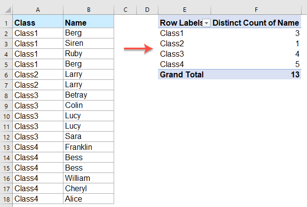
By default, when creating a pivot table based on a range of data containing duplicate values, all records are counted as well. However, sometimes we just want to count the unique values based on one column to get the result as the right screenshot shown. In this article, I will talk about how to count the unique values in a pivot table.
Count unique values in pivot table with Value Field Settings in Excel
Count unique values in pivot table with helper column (for Excel versions older than 2013)
Count unique values in pivot table with Value Field Settings
In Excel 2013 and later versions, a new Distinct Count function has been added in the pivot table, you can apply this feature to quickly and easily solve this task.
1. Select your data range and click Insert > PivotTable, in the Create PivotTable dialog box, choose a new worksheet or existing worksheet where you want to place the pivot table at, and check Add this data to the Data Model checkbox, see screenshot:

2. Then in the PivotTable Fields pane, drag the Class field to the Row box, and drag the Name field to the Values box, see screenshot:

3. And then click the Count of Name drop down list, choose Value Field Settings, see screenshot:

4. In the Value Field Settings dialog, click Summarize Values By tab, and then scroll to click Distinct Count option, see screenshot:

5. And then click OK, you will get the pivot table which count only the unique values.
- Note: If you check Add this data to the Data Model option in the Create PivotTable dialog box, the Calculated Field function will be disabled.
Count unique values in pivot table with helper column (for Excel versions older than 2013)
In older Excel versions, you need to create a helper column to identify the unique values, please do with the following steps:
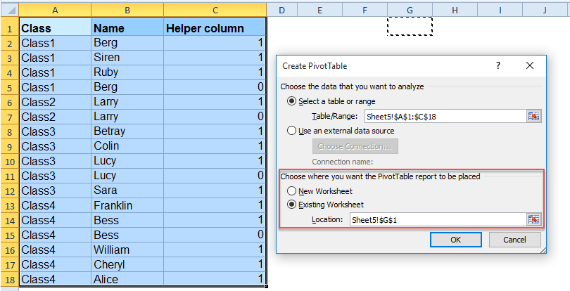
1. In a new column besides the data, please enter this formula =IF(SUMPRODUCT(($A$2:$A2=A2)*($B$2:$B2=B2))>1,0,1) into cell C2, and then drag the fill handle over the range of cells to apply this formula. The unique values will be identified, as shown in the screenshot below.

2. Now, you can create a pivot table. Select the data range including the helper column, then click Insert > PivotTable > PivotTable, see screenshot:

3. Then in the Create PivotTable dialog, choose a new worksheet or existing worksheet where you want to place the pivot table at, see screenshot:
4. Click OK, then drag the Class field to Row Labels box, and drag the Helper column field to Values box, and you will get a pivot table that counts only the unique values.

More relative PivotTable articles:
- Apply The Same Filter To Multiple Pivot Tables
- Sometimes, you may create several pivot tables based on the same data source, and now you filter one pivot table and want other pivot tables are filtered with the same way as well, that means, you want to change multiple pivot table filters at once in Excel. This article, I will talk about the usage of a new feature Slicer in Excel 2010 and later versions.
- Group Date By Month, Year, Half Year Or Other Specific Dates In Pivot Table
- In Excel, if the data in a pivot table includes date, and have you tried to group the data by month, quarter or year? Now, this tutorial will tell you how to group date by month/year/quarter in pivot table in Excel.
- Update Pivot Table Range In Excel
- In Excel, when you remove or add rows or columns in your data range, the relative pivot table does not update at the same time. Now this tutorial will tell you how to update the pivot table when rows or columns of the data table change.
- Hide Blank Rows In PivotTable In Excel
- As we know, pivot table is convenient for us to analyze the data in Excel, but sometimes, there are some blank contents appearing in the rows as below screenshot show. Now I will tell you how to hide these blank rows in pivot table in Excel.
Best Office Productivity Tools
Supercharge Your Excel Skills with Kutools for Excel, and Experience Efficiency Like Never Before. Kutools for Excel Offers Over 300 Advanced Features to Boost Productivity and Save Time. Click Here to Get The Feature You Need The Most...
Office Tab Brings Tabbed interface to Office, and Make Your Work Much Easier
- Enable tabbed editing and reading in Word, Excel, PowerPoint, Publisher, Access, Visio and Project.
- Open and create multiple documents in new tabs of the same window, rather than in new windows.
- Increases your productivity by 50%, and reduces hundreds of mouse clicks for you every day!
All Kutools add-ins. One installer
Kutools for Office suite bundles add-ins for Excel, Word, Outlook & PowerPoint plus Office Tab Pro, which is ideal for teams working across Office apps.
- All-in-one suite — Excel, Word, Outlook & PowerPoint add-ins + Office Tab Pro
- One installer, one license — set up in minutes (MSI-ready)
- Works better together — streamlined productivity across Office apps
- 30-day full-featured trial — no registration, no credit card
- Best value — save vs buying individual add-in