
How to highlight/conditional formatting dates older than 30 days in Excel?

For a list of date and you want to highlight the date cells that are older than 30 days since now, would you highlight them one by one manually? This tutorial introduces how to highlight dates older than 30 days with Conditional Formatting in Excel, and easily select and count dates older than a specific date with an amazing tool.

Highlight dates older than 30 days with conditional formatting
Easily select and highlight dates older than a specific date with an amazing tool

More tutorials for highlighting cells...


Easily select and count dates older than a specific date in Excel:

The Select Specific Cells utility of Kutools for Excel can help you quickly count and select all dates in a range of date cells which are older than a specific date in Excel. Download the full feature 30-day free trail of Kutools for Excel now!


Highlight dates older than 30 days with conditional formatting

With Excel’s Conditional Formatting function, you can quickly highlight dates older than 30 days. Please do as follows.

1. Select the dates data and click Home > Conditional Formatting > New Rule. See screenshot:

2. In the New Formatting Rule dialog, you need to:

  • 2.1) Select Use a formula to determine which cells to format option in the Select a Rule Type section;
  • 2.2) Enter the below formula into the Format values where this formula is true box;
  • =A2<TODAY()-30
  • 2.3) Click the Format button and specify a fill color to highlight the date cells;
  • 2.4) Click the OK button. See screenshot:

Note: in the above formula, A2 the first cell of your selected range, and 30 indicates older than 30 days, you can change them as your need.

Now all dates older than 30 day since today are highlighted with specified fill color.

If there are blank cells in the date list, they will be highlighted as well. If you don’t want the empty cells to be highlighted, please go ahead to create another rule.

3. Select the date list again, click Home > Conditional Formatting > Manage Rules.

4. In the Conditional Formatting Rules Manager dialog box, click the New Rule button.

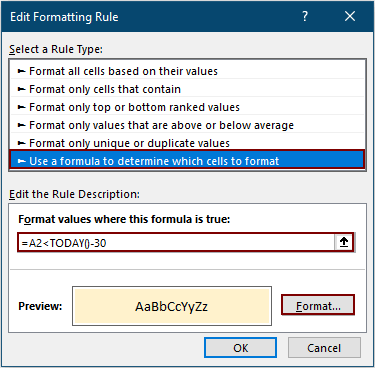
5. In the opening Edit Formatting Rule dialog box, please:

  • 5.1) Select Use a formula to determine which cells to format option in the Select a Rule Type section;
  • 5.2) Enter the below formula into the Format values where this formula is true box;
  • =ISBLANK(A2)=TRUE
  • 5.3) Click OK.

6. When it returns to the Conditional Formatting Rule Manager dialog box, you can see the rule is listed out, check the Stop if True box for it. And finally click the OK button.

Then you can see only dates older than 30 days in selected range are highlighted.


Easily highlight dates older than a specific date with an amazing tool

Here introduce a handy tool – Select Specific Cells utility of Kutools for Excel for you. With this utility, you can select all date cells in a certain range which is older than a specific date, and highlight it with background color manually as you need.

Before applying Kutools for Excel, please download and install it firstly.

1. Select the date cells, click Kutools > Select > Select Specific Cells.

2. In the Select Specific Cells dialog box, you need to:

  • 2.1) Select Cell in the Selection type section;
  • 2.2) Choose Less than from the Specific type drop-down list and enter a certain date you want to select all dates less than it into the text box;
  • 2.3) Click the OK button.
  • 2.4) Click OK in the next popping up dialog box. (This dialog box informs you how many cells match the condition and selected.)

3. After selecting the date cells, if you need to highlight them, please manually go to Home > Fill Color to specify a highlight color for them.

  If you want to have a free trial (30-day) of this utility, please click to download it, and then go to apply the operation according above steps.


Relative Articles:

Conditional format dates less than/greater than today in Excel
This tutorial shows you how to use the TODAY function in conditional formatting to highlight due dates or future dates in Excel in details.

Ignore blank or zero cells in conditional formatting in Excel
Supposing you have a list of data with zero or blank cells, and you want to conditional format this list of data but ignore the blank or zero cells, what would you do? This article will do you a favor.

Copy conditional formatting rules to another worksheet/workbook
For example you have conditionally highlighted entire rows based on duplicate cells in the second column (Fruit Column), and colored the top 3 values in the fourth column (Amount Column) as below screenshot shown. And now you want to copy the conditional formatting rule from this range to another worksheet/workbook. This article comes up with two workarounds to help you.

Highlight cells based on length of text in Excel
Supposing you are working with a worksheet which has list of text strings, and now, you want to highlight all the cells that the length of the text is greater than 15. This article will talks about some methods for solving this task in Excel.

More tutorials for highlighting cells...

Best Office Productivity Tools

🤖 Kutools AI Aide: Revolutionize data analysis based on: Intelligent Execution   |  Generate Code  |  Create Custom Formulas  |  Analyze Data and Generate Charts  |  Invoke Kutools Functions
Popular Features: Find, Highlight or Identify Duplicates   |  Delete Blank Rows   |  Combine Columns or Cells without Losing Data   |   Round without Formula ...
Super Lookup: Multiple Criteria VLookup    Multiple Value VLookup  |   VLookup Across Multiple Sheets   |   Fuzzy Lookup ....
Advanced Drop-down List: Quickly Create Drop Down List   |  Dependent Drop Down List   |  Multi-select Drop Down List ....
Column Manager: Add a Specific Number of Columns  |  Move Columns  |  Toggle Visibility Status of Hidden Columns  |  Compare Ranges & Columns ...
Featured Features: Grid Focus   |  Design View   |   Big Formula Bar    Workbook & Sheet Manager   |  Resource Library (Auto Text)   |  Date Picker   |  Combine Worksheets   |  Encrypt/Decrypt Cells    Send Emails by List   |  Super Filter   |   Special Filter (filter bold/italic/strikethrough...) ...
Top 15 Toolsets12 Text Tools (Add Text, Remove Characters, ...)   |   50+ Chart Types (Gantt Chart, ...)   |   40+ Practical Formulas (Calculate age based on birthday, ...)   |   19 Insertion Tools (Insert QR Code, Insert Picture from Path, ...)   |   12 Conversion Tools (Numbers to Words, Currency Conversion, ...)   |   7 Merge & Split Tools (Advanced Combine Rows, Split Cells, ...)   |   ... and more

Supercharge Your Excel Skills with Kutools for Excel, and Experience Efficiency Like Never Before. Kutools for Excel Offers Over 300 Advanced Features to Boost Productivity and Save Time.  Click Here to Get The Feature You Need The Most...

Description


Office Tab Brings Tabbed interface to Office, and Make Your Work Much Easier

  • Enable tabbed editing and reading in Word, Excel, PowerPoint, Publisher, Access, Visio and Project.
  • Open and create multiple documents in new tabs of the same window, rather than in new windows.
  • Increases your productivity by 50%, and reduces hundreds of mouse clicks for you every day!
Comments (22)
No ratings yet. Be the first to rate!
This comment was minimized by the moderator on the site
I got a solution to make the rest of the cells blank if they do not have a date or value in them.
Make a new rule. Select rule type: Format only cells that contain"
Choose "Format only cells with: Blanks:"
Then format it with a white background, or color of your excel spreadsheet. That should make all blanks turn white. Leaving the other dates that are over 30 days stay red. 
This comment was minimized by the moderator on the site
in support of my solution
This comment was minimized by the moderator on the site
I want solution. i want a formula through which if the date changed in 1 column then text and colour on the other column should be change by itself.can any body help me on this issue
This comment was minimized by the moderator on the site
I tried this, and it somewhat worked for me. The problem I have is the empty cells are still highlighted. I don't want the empty cells highlighted. What do I need to do to exclude the blank cells?
This comment was minimized by the moderator on the site
This happened to me as well, a couple of things to double check.1) the "STOP IF TRUE" box next to your rule in the rule manager is checked. 2) Make sure your 'applies to' for this rule is the same as the one for the other rule(s) 3) Check your formula and subculture the "A2" with what matches the column that you are creating the rule for. For example, for my table all of my dates are in the column J and the dates start in row 7 so my formula for this would be =ISBLANK(J7)=TRUE
I hope that this helps!
This comment was minimized by the moderator on the site
It doesn't work well, only the cell L1 is formated and no other one. Only the cell L1 is marked with an other backround color. Pleas add also when and which cells should be marked before clicking on "new rule."
This comment was minimized by the moderator on the site
The issue with less than 30 days is, it is even high

lighting blank cells.
This comment was minimized by the moderator on the site
Hi there, I've searched far and low and have not yet found the specific formatting that I'm looking for. I would like to be able to have a list of all the 5th Sundays in the month, per specific year(There are always 4 months that have 5 Sundays every year).

So since I don't know how to do that, I have a function that looks at dates (Jan - Dec of a year) and finds the first Sunday of the month, then adds 4 weeks to that, which would give me the 5th Sunday of the month.

=DATE(YEAR(A2),MONTH(A2),1+((5-(1>=WEEKDAY(DATE(YEAR(A2),MONTH(A2),1))))*7)+(1-WEEKDAY(DATE(YEAR(A2),MONTH(A2),1))))

So some months the resulting dates actually show up in the next month - well all of the ones that don't have 5 Sundays.
So now I was thinking if I could at least have conditional formatting where the "DAY" value in the date is above a certain number, then I could at least easily highlight the ones that have 5 Sundays. But I have not been able to figure it out. Can someone help me with that? It seems to me it should be simple to have a conditional formatting that highlights all the days that are after the middle of the month, regardless of which month or year it is.
This comment was minimized by the moderator on the site
I am using the Highlighting function with dates greater than 90 days, but then I have a completed date that I would like to use that will remove the highlight when a date is added to this cell. Example Due Date - Highlighted Cell - Completed Date. Is there a formula that will do this?
This comment was minimized by the moderator on the site
Is it possible to compare 2 dates like; (first date > (second date+5)), and condition a cell colour based on the result?
This comment was minimized by the moderator on the site
Yes, you just need to compare the cells $n$m>,<,=$o$p


Let me know if it works or else, I will provide you another video


Reach me out
This comment was minimized by the moderator on the site
I got the above down but what if I only wanted to count weekdays? No weekends or holidays.
There are no comments posted here yet
Load More
Please leave your comments in English
Posting as Guest
×
Rate this post:
0   Characters
Suggested Locations