How to make row labels on same line in pivot table?

After creating a pivot table in Excel, you will see the row labels are listed in only one column. But, if you need to put the row labels on the same line to view the data more intuitively and clearly as following screenshots shown. How could you set the pivot table layout to your need in Excel?
Make row labels on same line with setting the layout form in pivot table
If you want to follow along with this tutorial, please download the example spreadsheet.

Make row labels on same line with setting the layout form in pivot table
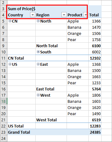
As we all know, the pivot table has several layout form, the tabular form may help us to put the row labels next to each other. Please do as follows:
1. Click any cell in your pivot table, and the PivotTable Tools tab will be displayed.
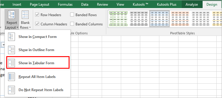
2. Under the PivotTable Tools tab, click Design > Report Layout > Show in Tabular Form, see screenshot:
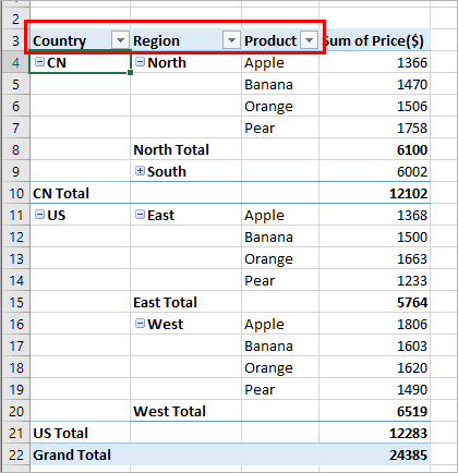
3. And now, the row labels in the pivot table have been placed side by side at once, see screenshot:
Group PivotTable Data by Sepcial Time
The PivotTable Special Time Grouping in Kutools for Excel supports following operations which Excel's bult-in functions cannot support:
- Group data by fiscal year in Pivot Table
- Group data by half year in Pivot Table
- Group data by week number in Pivot Table
- Group data by day of week in Pivot Table
- Group data by half hour or specific minutes in Pivot Table
Kutools for Excel: a handy add-in with more than 300 advanced tools solves your 90% puzzels in Excel.
Make row labels on same line with PivotTable Options
You can also go to the PivotTable Options dialog box to set an option to finish this operation.
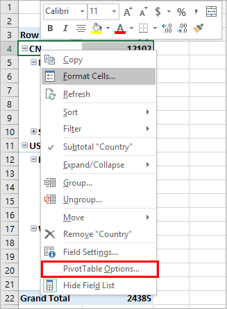
1. Click any one cell in the pivot table, and right click to choose PivotTable Options, see screenshot:
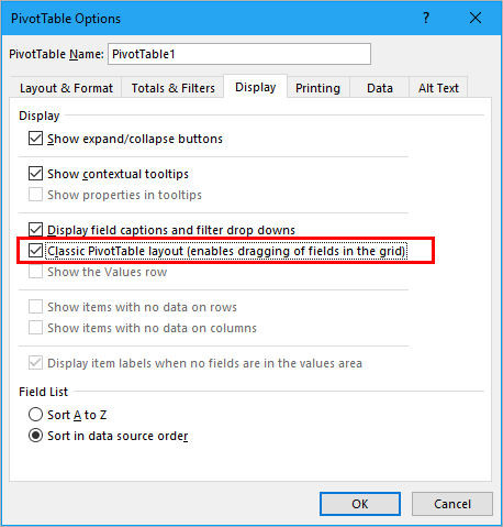
2. In the PivotTable Options dialog box, click the Display tab, and then check Classic PivotTable layout(enables dragging of fields in the grid) option, see screenshot:
3. Then click OK to close this dialog, and you will get the following pivot table which row labels are separated in different columns.
Relative Articles:
How to add average/grand total line in a pivot chart in Excel?
In this article I will share a tricky way to add an average/grand total line in a pivot chart as normal chart in Excel easily.
How to filter Pivot table based on a specific cell value in Excel?
Normally, we are filtering data in a Pivot Table by checking values from the drop-down list. If you want to make a Pivot Table more dynamic by filtering, you can try to filter it based on value in a specific cell. The VBA method in this article will help you solving the problem.
How to count unique values in pivot table?
By default, when we create a pivot table based on a range of data which contains some duplicate values, all the records will be counted. But,sometimes, we just want to count the unique values based on one column to get the second screenshot result. In this article, I will talk about how to count the unique values in pivot table.
How to clear old items in pivot table?
After creating the pivot table based on a data range, sometimes, we need to change the data source to our need. But, the old items might still reserve in the filter drop down, this will be annoying. In this article, I will talk about how to clear the old items in pivot table.
How to repeat row labels for group in pivot table?
In Excel, when you create a pivot table, the row labels are displayed as a compact layout, all the headings are listed in one column. Sometimes, you need to convert the compact layout to outline form to make the table more clearly. This article will tell you how to repeat row labels for group in Excel PivotTable.
Best Office Productivity Tools
Supercharge Your Excel Skills with Kutools for Excel, and Experience Efficiency Like Never Before. Kutools for Excel Offers Over 300 Advanced Features to Boost Productivity and Save Time. Click Here to Get The Feature You Need The Most...
Office Tab Brings Tabbed interface to Office, and Make Your Work Much Easier
- Enable tabbed editing and reading in Word, Excel, PowerPoint, Publisher, Access, Visio and Project.
- Open and create multiple documents in new tabs of the same window, rather than in new windows.
- Increases your productivity by 50%, and reduces hundreds of mouse clicks for you every day!
All Kutools add-ins. One installer
Kutools for Office suite bundles add-ins for Excel, Word, Outlook & PowerPoint plus Office Tab Pro, which is ideal for teams working across Office apps.
- All-in-one suite — Excel, Word, Outlook & PowerPoint add-ins + Office Tab Pro
- One installer, one license — set up in minutes (MSI-ready)
- Works better together — streamlined productivity across Office apps
- 30-day full-featured trial — no registration, no credit card
- Best value — save vs buying individual add-in