How to Create a Bubble Chart with Multiple Series in Excel
A bubble chart makes it easy to compare multiple items, with the size of each bubble helping highlight differences in values such as market share. However, creating a chart in which each item appears as a separate series can require considerable manual setup in Excel.
This article explains how to create a bubble chart with multiple series manually in Excel and how to create one more quickly with Kutools for Excel.
- Create a bubble chart with multiple series using Excel’s built-in chart tools.
- Quickly create a bubble chart with multiple series using Kutools for Excel.
Comparison of the methods
| Feature | Excel built-in method | Kutools for Excel |
|---|---|---|
| Creates multiple series | Yes | Yes |
| Automatically identifies data fields | No | Yes |
| Requires adding series individually | Yes | No |
| Supports Bubble and 3-D Bubble styles | Yes | Yes |
| Data label options available during setup | No | Yes |
| Setup effort | High | Low |
| Best for | Manually controlling each series | Quickly creating a chart from structured data |
The built-in Excel method provides full control over each individual series but requires more setup. Kutools is more convenient when the source data is already arranged in columns and you want to create the entire chart at once.
Create a bubble chart with multiple series using Excel’s built-in tools
Excel can create a bubble chart with multiple series, but each series must be added and configured separately.
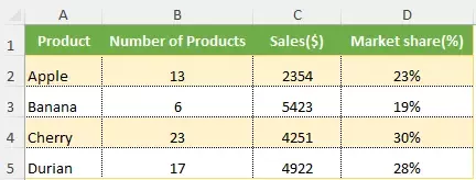
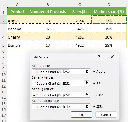
Before starting, arrange the source data into four columns containing the series names, X values, Y values, and bubble sizes, as shown in the screenshot below.
Step 1: Insert a blank bubble chart
- Click a blank cell outside the source data.
- Go to the Insert tab.
- Click Insert Scatter (X, Y) or Bubble Chart.
- Under Bubble, select Bubble or 3-D Bubble.
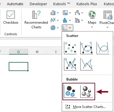
A blank chart is inserted into the worksheet.
Step 2: Open the Select Data Source dialog box
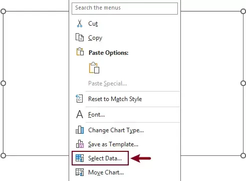
Right-click the blank chart and select Select Data from the context menu.
Step 3: Add the first series
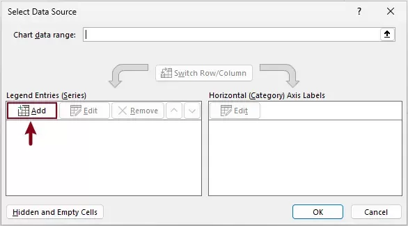
- In the Select Data Source dialog box, click Add under Legend Entries (Series).
- In the Edit Series dialog box, configure the following fields:
- Series name: Select the cell containing the name of the first series.
- Series X values: Select the cell containing its X value.
- Series Y values: Select the cell containing its Y value.
- Series bubble size: Select the cell containing the value that determines the bubble size.
- Click OK to add the series.
Step 4: Add the remaining series
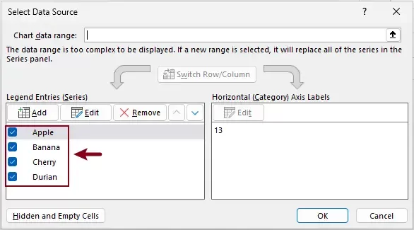
Repeat Step 3 for every remaining data row. Each row must be added as a separate series if you want it to appear independently in the chart legend.
After all the series have been added, click OK to close the Select Data Source dialog box.
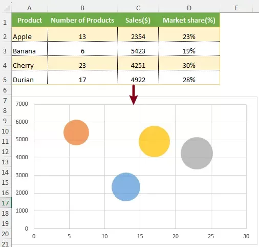
The bubble chart with multiple series is now created.
Tips:
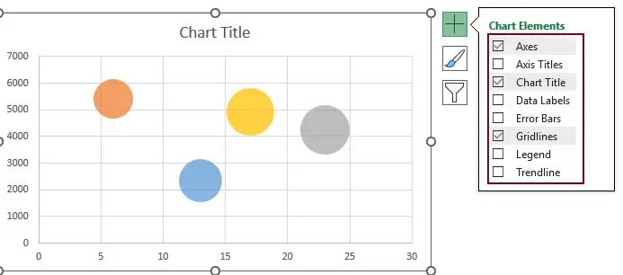
- After creating the chart, select it and click the Chart Elements (+) button in the upper-right corner to add or adjust the chart title, legend, data labels, axes, and other chart elements.
- Creating many series manually can take considerable time because the series name, X value, Y value, and bubble size must be specified separately for every series.
Quickly create a bubble chart with multiple series using Kutools for Excel
Adding every series individually can be inefficient when the source table contains many rows. The Bubble Chart feature in Kutools for Excel automatically identifies the selected data fields and creates a multiple-series bubble chart without requiring you to add each series manually.
Kutools for Excel - Packed with over 300 essential tools for Excel. Make Excel tasks faster, easier, and more efficient. Download now!
Step 1: Select the source data
Select the entire data range, including the column headings.
Step 2: Open the Bubble Chart feature
Click Kutools > Charts > Data Distribution > Bubble Chart.
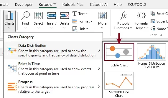
Step 3: Check the chart settings and create the chart
In the Create bubble chart dialog box, Kutools automatically identifies the selected table and fills in the required fields. Check the selected data ranges, and then click OK to create the bubble chart.
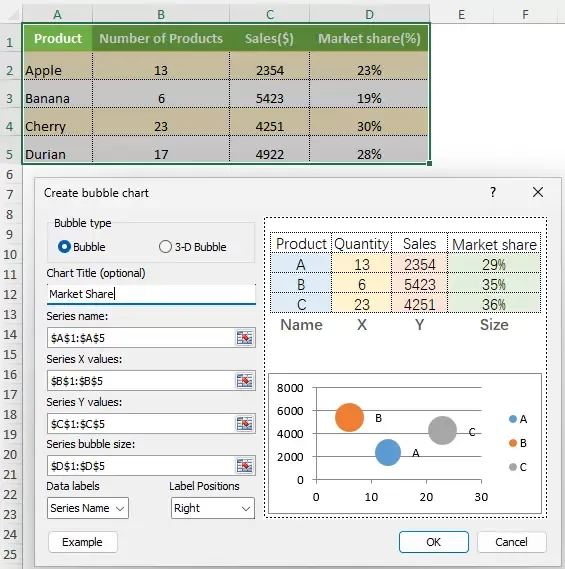
Tip: You can also configure the following options before creating the chart:
- Under Bubble type, select Bubble or 3-D Bubble.
- Enter a chart title in Chart Title (optional) if needed.
- Select the content to display from the Data labels list.
- Choose where the data labels appear from the Label Positions list.
Result
Kutools immediately creates a bubble chart in which each selected data row is displayed as a separate series.
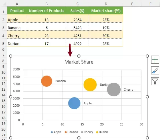
Kutools for Excel - Supercharge Excel with over 300 essential tools, making your work faster and easier, and take advantage of AI features for smarter data processing and productivity. Get It Now
Frequently Asked Questions
Conclusion
Excel’s built-in chart tools can create a bubble chart with multiple series, but each series must be added and configured individually. This method is suitable when you need precise control over every series and do not mind the additional setup.
For a faster solution, the Bubble Chart feature in Kutools for Excel automatically matches the series names, X values, Y values, and bubble sizes from the selected table. It can create a standard or 3-D bubble chart in only a few steps, making it especially useful for datasets containing many series.
Best Office Productivity Tools
Supercharge Your Excel Skills with Kutools for Excel, and Experience Efficiency Like Never Before. Kutools for Excel Offers Over 300 Advanced Features to Boost Productivity and Save Time. Click Here to Get The Feature You Need The Most...
Office Tab Brings Tabbed interface to Office, and Make Your Work Much Easier
- Enable tabbed editing and reading in Word, Excel, PowerPoint, Publisher, Access, Visio and Project.
- Open and create multiple documents in new tabs of the same window, rather than in new windows.
- Increases your productivity by 50%, and reduces hundreds of mouse clicks for you every day!
All Kutools add-ins. One installer
Kutools for Office suite bundles add-ins for Excel, Word, Outlook & PowerPoint plus Office Tab Pro, which is ideal for teams working across Office apps.





- All-in-one suite — Excel, Word, Outlook & PowerPoint add-ins + Office Tab Pro
- One installer, one license — set up in minutes (MSI-ready)
- Works better together — streamlined productivity across Office apps
- 30-day full-featured trial — no registration, no credit card
- Best value — save vs buying individual add-in
Table of contents
- Method comparison
- Create a bubble chart with Excel built-in
- Quickly create a bubble chart with Kutools
- Frequently Asked Questions
- Conclusion
- The Best Office Productivity Tools
Kutools for Excel
Brings 300+ powerful features to streamline your Excel tasks.
- ⬇️ Free Download
- 🛒 Purchase Now
- 📘 Feature Tutorials
- 🎁 30-Day Free Trial