How to create a bell curve chart template in Excel?
The bell curve chart, also known as the normal distribution or Gaussian distribution in statistics, is a widely used graph to depict data distributions where most values cluster around the mean, highlighting the probability of different outcomes. The highest point of the curve represents the most probable event. Such charts are commonly used in fields like quality control, exam score analysis, business performance evaluation, and more, as they provide intuitive visual insight into the distribution and likelihood of observed values. This article will walk you through step-by-step instructions to create a bell curve chart using your own dataset in Excel and further guide you on how to save this setup as a reusable chart template for future analyses.
- Create a bell curve chart and save as chart template in Excel
- Quickly create a bell curve with an amazing tool
- VBA: Generate bell curve chart with code (alternative solution)
Create a bell curve chart and save as a chart template in Excel
Creating a bell curve in Excel is a multi-step process, but once set up, you can customize the chart for various datasets or save the design for repeated use. This solution gives you full control over the data, calculation methods, and visual formatting—ideal if you need a precise, customizable chart for in-depth data analysis.
Advantages: Maximum flexibility; all steps are clearly visible for learning or documentation needs.
Disadvantages: Requires manual calculation steps and careful attention to formulas.
Follow these detailed steps:
1. Open a new Excel workbook, and create column headers in Range A1:D1 as shown in the screenshot below. The recommended headers are: Data, Distribution, Mean, Standard Deviation.
2. Input your source numbers under the "Data" column. For best bell curve appearance, your data should cover a wide range and be sufficiently numerous (at least 30–50 values recommended). For our example, we enter values from 10 to 100 in A2:A92.
To ensure the data is arranged from smallest to largest, select your number-filled cells in column A and click Data > Sort A to Z. This helps the plotted curve form correctly.
3. Calculate supporting statistics:
(1) In cell C2, enter the following formula to calculate the arithmetic average (mean) of your dataset:
This function takes the average of the selected range. Make sure your range matches your actual data, or adjust as needed.
(2) In cell D2, calculate the standard deviation, which is used to shape the width of the bell curve:
Note: In recent Excel versions, =STDEV.S() may also be suggested for sample standard deviation.
(3) In B2, generate the probability distribution for each data point. Depending on Excel version, use one of these formulas:
A. For Excel2010 or later: =NORM.DIST(A2,$C$2,$D$2,FALSE) | B. For Excel2007: =NORMDIST(A2,$C$2,$D$2,FALSE) |
Enter the appropriate formula in cell B2. Then, drag the AutoFill Handle down to fill the formula for all data rows (up to B92 in this example). This creates the distribution (bell curve) value for each original data point.
Note: If your dataset covers a different range, update all cell references in the formulas accordingly. Also, errors in formula application often result from an incorrect range or cell misplacement, so double-check references. 
4. Highlight both the Data and Distribution columns (e.g., Range A2:B92). Go to Insert > Scatter (or Scatter and Doughnut chart in Excel 2013+) > Scatter with Smooth Lines and Markers. This chart type best visualizes the bell-shaped pattern.

The chart now displays your bell curve, similar to the following example:
For clarity and aesthetics, you may want to remove unnecessary chart elements such as gridlines, axis labels, or legends to spotlight the bell shape. Right-click the element you wish to remove and select “Delete” or uncheck it from the chart formatting options.
To reuse this chart with other data, you should save it as a template:
5. Save the bell curve as a chart template:
A. In Excel 2013 or later: Right-click the completed bell curve chart, select Save as Template from the menu.
B. In Excel 2007/2010: Click the chart to enable Chart Tools, then go to Design > Save As Template.
This allows faster creation of new bell curves for other datasets in the future without repeating all formatting.
6. When the Save Chart Template dialog appears, specify a recognizable name in the File name field (for example, "BellCurveTemplate"), and click Save. This template is stored in the default "Templates" folder, usually accessible under the chart selection dialog for new workbooks.
Troubleshooting tips:
- If the template save option is unavailable, ensure the chart is selected and that you have proper permissions to write files in the default template folder.
- If future charts don't resemble your saved bell curve, double-check the input data for completeness and proper formatting.
Quickly create a bell curve with an amazing tool
If you want to bypass manual calculations and complex formulas, Kutools for Excel provides a Normal Distribution / Bell Curve feature that creates professional-looking bell curve charts in just a few clicks. This method is especially valuable when you're working with unfamiliar data or require an immediate statistical visual without deep knowledge of Excel functions.
Advantages: Drastically reduces the time and skill required to create bell curve or combination charts. Includes extra options such as frequency histogram and combo charts for more comprehensive analysis.
Disadvantages: Requires installation of Kutools for Excel.
1. Select the range containing your data values. Make sure your data is numeric and does not contain blank cells or text for optimal results. Click Kutools > Charts > Data Distribution > Normal Distribution / Bell Curve.
2. In the dialog box that appears, select the Normal distribution chart option under the Select section. Click OK to create the chart.
This dialog also allows you to:
(1) Optionally input a chart title for immediate labeling.
(2) Create a frequency histogram by checking only Frequency histogram chart.
(3) Combine a histogram and bell curve in one visual by checking both options under Select.
If only the Normal Distribution chart option is chosen:
If both Normal Distribution chart and Frequency histogram chart are checked for a combo effect:
Precautions:
- Ensure data range contains only valid numeric entries.
- If the resulting chart does not appear as expected, check for data errors or range mismatches.
Compared to manual solutions, using Kutools for Excel is ideal for quick and consistent results, especially when producing charts for reports or presentations with minimal effort.
VBA: Automatically generate a bell curve with a macro
For advanced users or those automating repetitive reporting, a simple VBA macro can quickly generate bell curve data from user-defined parameters and plot the graph automatically. This is especially helpful when working with changing data or for frequent reporting that requires consistent format.
Advantages: Can automate both calculation and chart creation; good for batch processing.
Disadvantages: Some familiarity with macros is needed and may require security permissions to run VBA scripts.
- Prepare your data.If you already have a dataset (e.g., in range A2:A92), calculate the mean, standard deviation, range start/end using Excel formulas:Get the mean:
=AVERAGE(A2:A92)Get the Standard Deviation:=STDEV.P(A2:A92)Get the Range Start:=Mean-3*Standard DeviationAs the mean is in B2, Standard Deviation is in C2, this formula should be: =B2-3*C2Get the Range End:=Mean+3*Standard DeviationAs the mean is in B2, Standard Deviation is in C2, this formula should be: =B2+3*C2For the step, use 1 or 0.1. The smaller the step value, the smoother the curve becomes.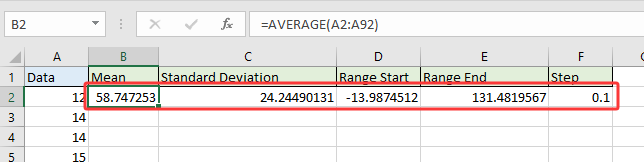
- Run the code
- Press Alt + F11 to open the VBA editor.
- Insert a new module and paste the GenerateBellCurve macro code.
Sub GenerateBellCurve() 'Updated by Extendoffice 2025/07/24 Dim xMean As Double Dim xStdev As Double Dim xStart As Double Dim xEnd As Double Dim xStep As Double Dim xRow As Integer Dim ws As Worksheet Dim chartObj As ChartObject Dim xValue As Double On Error Resume Next xTitleId = "KutoolsforExcel" Set ws = Worksheets.Add ws.Name = "BellCurve" xMean = Application.InputBox("Enter mean value:", xTitleId, 50, Type:=1) xStdev = Application.InputBox("Enter standard deviation:", xTitleId, 10, Type:=1) xStart = Application.InputBox("Enter range start (e.g. 10):", xTitleId, xMean - 3 * xStdev, Type:=1) xEnd = Application.InputBox("Enter range end (e.g. 100):", xTitleId, xMean + 3 * xStdev, Type:=1) xStep = Application.InputBox("Enter step interval (e.g. 1):", xTitleId, 1, Type:=1) ws.Range("A1:B1").Value = Array("X", "Normal Distribution") xRow = 2 For xValue = xStart To xEnd Step xStep ws.Cells(xRow, 1).Value = xValue ws.Cells(xRow, 2).Value = WorksheetFunction.Norm_Dist(xValue, xMean, xStdev, False) xRow = xRow + 1 Next Set chartObj = ws.ChartObjects.Add(Left:=300, Width:=500, Top:=10, Height:=300) With chartObj.Chart .ChartType = xlXYScatterSmooth .SetSourceData Source:=ws.Range("A1:B" & xRow - 1) .HasTitle = True .ChartTitle.Text = "Bell Curve" .Axes(xlCategory).HasTitle = True .Axes(xlCategory).AxisTitle.Text = "X" .Axes(xlValue).HasTitle = True .Axes(xlValue).AxisTitle.Text = "Probability Density" End With ws.Activate End Sub - Press F5 to run the macro.
- Enter the Required Values When PromptedThe macro will ask for:
- Mean value: Just select the cell containing the mean value you have calculated. You can manually enter the value if you remember it.
- Standard deviation: Select the cell containing the Standard deviation.
- Range start: Select the cell containing the range start.
- Range end: Select the cell containing the range end
- Step: Enter 1 or 0.1. Or select the cell containing the step value.

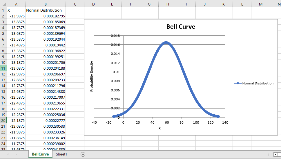
Once complated, a new worksheet name BellCurve will be created.
- Column A contains the X-axis values (data range).
- Column B contains probability density values calculated using NORM.DIST().
- A smooth scatter chart (bell curve) will be inserted directly in the worksheet.

Tip: If an error occurs, recheck the parameter inputs and ensure you have permissions to add worksheets and charts. Always save your work before running VBA scripts as macros may not be undone.
Related Articles

Move chart X axis below negative values/zero/bottom in Excel
When negative data existing in source data, the chart X axis stays in the middle of chart. For good looking, some users may want to move the X axis below negative labels, below zero, or to the bottom in the chart in Excel.

Add a horizontal average line to chart in Excel
In Excel, you may often create a chart to analyze the trend of the data. But sometimes, you need to add a simple horizontal line across the chart that represents the average line of the plotted data, so that you can see the average value of the data clearly and easily.

Break chart axis in Excel
When there are extraordinary big or small series/points in source data, the small series/points will not be precise enough in the chart. In these cases, some users may want to break the axis, and make both small series and big series precise simultaneously.
Best Office Productivity Tools
Supercharge Your Excel Skills with Kutools for Excel, and Experience Efficiency Like Never Before. Kutools for Excel Offers Over 300 Advanced Features to Boost Productivity and Save Time. Click Here to Get The Feature You Need The Most...
Office Tab Brings Tabbed interface to Office, and Make Your Work Much Easier
- Enable tabbed editing and reading in Word, Excel, PowerPoint, Publisher, Access, Visio and Project.
- Open and create multiple documents in new tabs of the same window, rather than in new windows.
- Increases your productivity by 50%, and reduces hundreds of mouse clicks for you every day!
All Kutools add-ins. One installer
Kutools for Office suite bundles add-ins for Excel, Word, Outlook & PowerPoint plus Office Tab Pro, which is ideal for teams working across Office apps.
- All-in-one suite — Excel, Word, Outlook & PowerPoint add-ins + Office Tab Pro
- One installer, one license — set up in minutes (MSI-ready)
- Works better together — streamlined productivity across Office apps
- 30-day full-featured trial — no registration, no credit card
- Best value — save vs buying individual add-in