How to perform vlookup across multiple worksheets?
VLOOKUP is one of the most widely used functions in Excel for searching and retrieving data. However, when dealing with multiple worksheets, a direct VLOOKUP function won’t suffice since it works within a single range. Supposing I have the following three worksheets with range of data, and now, I want to get part of the corresponding values based on the criteria from these three worksheets. This guide explains how to implement a multi-worksheet VLOOKUP in Excel using various methods.
 |  |  |  |
Vlookup values from multiple worksheets by an array formula
Vlookup values from multiple worksheets by Kutools for Excel
Vlookup values from multiple worksheets by a normal formula
Vlookup values from multiple worksheets by an array formula
To use this array formula, you should give these three worksheets a range name, please list your worksheet names in a new worksheet, such as following screenshot shown:

1. Give these worksheets a range name, select the sheet names, and type a name in the Name Box which next to the formula bar, in this case, I will type Sheetlist as the range name, and then press Enter key.

2. And then you can enter the following long formula into your specific cell:
=VLOOKUP(A2,INDIRECT("'"&INDEX(Sheetlist,MATCH(1,--(COUNTIF(INDIRECT("'"&Sheetlist&"'!$A$2:$B$6"),A2)>0),0))&"'!$A$2:$B$6"),2,FALSE)3. And then, press Ctrl + Shift + Enter keys together to get the first corresponding value, then drag the fill handle down to the cells that you want to apply this formula, all the relative values of each row have been returned as follows:

Notes:
1. In the above formula:
- A2: is the cell reference which you want to return its relative value;
- Sheetlist: is the range name of the worksheet names I have created in step1;
- A2:B6: is the data range of the worksheets you need to search;
- 2: indicates the column number that your matched value is returned.
2. If the specific value you lookup doesn't exist, a #N/A value will be displayed.
Vlookup values from multiple worksheets by Kutools for Excel
Kutools for Excel provides you with an efficient and simple feature - "LOOKUP Across Multiple Sheets" , helping you easily perform VLOOKUP queries across multiple worksheets. Without the need for complex formulas, you can quickly search and extract the required data from multiple sheets. With just a few clicks, you can complete the matching and integration of data from multiple tables, significantly improving work efficiency. Additionally, Kutools supports saving previously used schemes, making it convenient for direct use in future tasks.
After installing Kutools for Excel, please do as this:
1. Click "Kutools" > "Super Lookup" > "LOOKUP Across Multiple Sheets", see screenshot:

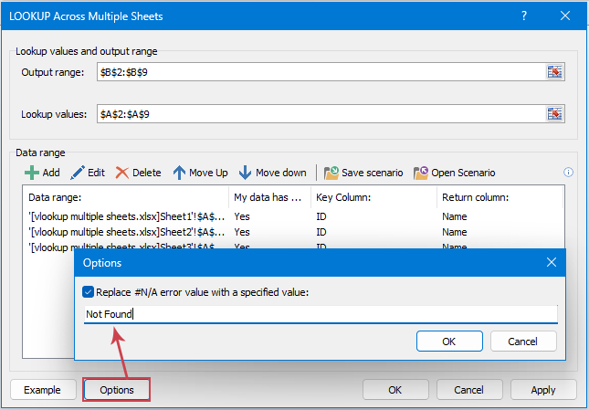
2. In the "LOOKUP Across Multiple Sheets" dialog box, please do the following operations:
- Select the output cells and lookup value cells from the "Output Range" and "Lookup values" section separately;
- Then, clcik "Add" button to select and add the data range from other sheets one by one into the "Data range" list box.
- Finally, click OK button.


Result: All the matching records have been returned, see screenshots:
| | |  |
Click to Download Kutools for Excel and free trial Now!
Vlookup values from multiple worksheets by a normal formula
If you do not want to make the range name and are not familiar with the array formula, here also has a normal formula to help you.
1. Please type the following formula into a cell you need:
=IFERROR(VLOOKUP($A2,Sheet1!$A$2:$B$6,2,FALSE),IFERROR(VLOOKUP($A2,Sheet2!$A$2:$B$6,2,FALSE),VLOOKUP($A2,Sheet3!$A$2:$B$6,2,FALSE)))2. And then drag the fill handle down to the range of cells you want to contain this formula, see screenshot:

Notes:
1. In the above formula:
- A2: is the cell reference which you want to return its relative value;
- Sheet1, Sheet2, Sheet3: are the sheet names which include the data you want to use;
- A2:B6: is the data range of the worksheets you need to search;
- 2: indicates the column number that your matched value is returned.
2. For much easier to understand this formula, in fact, the long formula is composed by several vlookup function and connect with the IFERROR function. If you have more worksheets, you just need to add the vlookup function in conjunction with the IFERROE after the formula.
3. If the specific value you lookup doesn't exist, a #N/A value will be displayed.
Conclusion:
This guide has provided three distinct methods to perform VLOOKUP across multiple worksheets, catering to various user needs and skill levels:
- Array Formula: A powerful method for advanced users, array formulas enable dynamic and flexible lookups across multiple sheets without the need for additional tools. While it requires a bit of formula expertise, it’s efficient and effective for complex datasets.
- Kutools for Excel: An excellent choice for users looking for a user-friendly, automated solution. With its built-in tools, Kutools simplifies the multi-sheet lookup process, saving time and effort, especially for those less familiar with Excel’s advanced functions.
- Normal Formula: Using nested IFERROR or IF formulas is a practical and straightforward way to achieve multi-sheet lookups. This approach is ideal for smaller datasets or when you need a quick solution without additional tools or advanced techniques.
Choosing the right method depends on your familiarity with Excel, the complexity of your task, and the tools at your disposal. If you're interested in exploring more Excel tips and tricks, our website offers thousands of tutorials to help you master Excel.
More relative articles:
- Vlookup Matching Value From Bottom To Top In Excel
- Normally, the Vlookup function can help you to find the data from top to bottom to get the first matching value from the list. But, sometimes, you need to vlookup from bottom to top to extract the last corresponding value. Do you have any good ideas to deal with this task in Excel?
- Vlookup And Return Whole / Entire Row Of A Matched Value In Excel
- Normally, you can vlookup and return a matching value from a range of data by using the Vlookup function, but, have you ever tried to find and return the whole row of data based on specific criteria as following screenshot shown.
- Vlookup And Concatenate Multiple Corresponding Values In Excel
- As we all known, the Vlookup function in Excel can help us to lookup a value and return the corresponding data in another column, but in general, it can only get the first relative value if there are multiple matching data. In this article, I will talk about how to vlookup and concatenate multiple corresponding values in only one cell or a vertical list.
- Vlookup Across Multiple Sheets And Sum Results In Excel
- Supposing, I have four worksheets which have the same formatting, and now, I want to find the TV set in the Product column of each sheet, and get the total number of order across those sheets as following screenshot shown. How could I solve this problem with an easy and quick method in Excel?
- Vlookup And Return Matching Value In Filtered List
- The VLOOKUP function can help you to find and return the first matching value by default whether it is a normal range or filtered list. Sometimes, you just want to vlookup and return only the visible value if there is a filtered list. How could you deal with this task in Excel?
Best Office Productivity Tools
Supercharge Your Excel Skills with Kutools for Excel, and Experience Efficiency Like Never Before. Kutools for Excel Offers Over 300 Advanced Features to Boost Productivity and Save Time. Click Here to Get The Feature You Need The Most...
Office Tab Brings Tabbed interface to Office, and Make Your Work Much Easier
- Enable tabbed editing and reading in Word, Excel, PowerPoint, Publisher, Access, Visio and Project.
- Open and create multiple documents in new tabs of the same window, rather than in new windows.
- Increases your productivity by 50%, and reduces hundreds of mouse clicks for you every day!