How to vlookup matching values from right to left in Excel?
The VLOOKUP function in Excel is widely used for searching and retrieving data. However, one of its limitations is that it can only look up values from left to right. This means the lookup value must be in the first column of the table, and the return value must be to the right of the lookup column. But what if you need to look up values from right to left? This guide will explore several methods to achieve this, including both formula-based and automated VBA solutions. Understanding and applying these right-to-left lookup techniques can help you effectively handle real-world data layouts that don't always fit the typical VLOOKUP requirements.
Vlookup values from right to left with VLOOKUP and IF functions
While VLOOKUP alone cannot look up values from right to left, you can manipulate your data structure using the IF function to make it work. This approach is especially handy if you prefer sticking with familiar Excel functions and want a quick solution without rearranging your actual dataset.
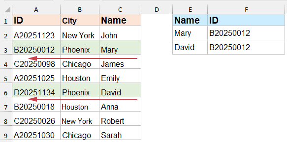
Please enter the formula below into the needed cell, and then drag the fill handle to the cells you want to apply this formula to get all the corresponding values. This approach is effective for static ranges but may require adjustment if your data expands or changes structure. See screenshot:
=VLOOKUP(E2, IF({1,0}, $C$2:$C$9, $A$2:$A$9), 2, 0)
- E2: This is the value you are looking for. It's the key that Excel will search for in the specified range.
- IF({1,0}, $C$2:$C$9, $A$2:$A$9): This part of the formula creates a virtual table by rearranging the columns. Normally, VLOOKUP can only search the first column of a table and return a value from a column to the right. By using IF({1,0}, ...), you are telling Excel to create a new table where the columns are swapped:
♦ The first column of the new table is $C$2:$C$9.
♦ The second column of the new table is $A$2:$A$9. - 2: This tells VLOOKUP to return the value from the second column of the virtual table created by the IF function. In this case, it will return a value from $A$2:$A$9.
- 0: This specifies that you want an exact match. If Excel doesn't find an exact match for E2 in $C$2:$C$9, it will return an error.
Tip: If you see a #N/A error, double-check that the lookup value exists in your lookup column. This approach is straightforward for simple (static range) lookups, but may be less suitable for large dynamic ranges or where table size or position changes often.
Vlookup values from right to left with Kutools for Excel
If you prefer a more user-friendly approach, Kutools for Excel offers advanced features that simplify complex lookups, including the ability to search from right to left effortlessly. Kutools is suitable for users who want to avoid complex formulas and have faster access to advanced search options without manual setup. This approach works well for data of all sizes and for those who regularly perform lookups.
After installing Kutools for Excel, please do as this:
1. Click "Kutools" > "Super Lookup" > "LOOKUP from Right to Left", see screenshot:

2. In the "LOOKUP from Right to Left" dialog box, please do the following operations:
- Select the lookup value cells and output cells from the "Output Range" and "Lookup values" sections;
- Then, specify the corresponding items from the "Data range" section. Make sure your ranges are accurate to avoid mismatches.
- Finally, click the OK button.


3. Now, the matching records have been returned based on the lookup values from the right list, see screenshot:

If you want to replace the #N/A error value with another text value, you just need to click the "Options" button and check the "Replace #N/A error value with a specified value" option, then type the text you need. 
This feature is particularly useful when sharing worksheets, as it prevents error messages from appearing in your final outputs.
Vlookup values from right to left with INDEX and MATCH functions
The combination of INDEX and MATCH is a versatile and powerful alternative to VLOOKUP. It allows you to look up values in any direction (left, right, up, or down), giving you greater flexibility, especially when your lookup column is not the first column in the data range. INDEX and MATCH are well-suited for larger datasets and for dynamic tables where column positions may change.
Enter or copy the formula below into a blank cell to output the result, then drag the fill handle down to your cells that you want to contain this formula. Make sure ranges cover your intended data and that you use absolute references (the $ sign) if you want to keep the lookup ranges fixed when copying down the formula.
=INDEX($A$2:$A$9,MATCH(E2,$C$2:$C$9,0))
- E2: This is the value you are looking for.
- MATCH(E2, $C$2:$C$9,0): The MATCH function searches for the value in E2 within the range $C$2:$C$9. The0 indicates that you want an exact match. If it finds the value, it returns the relative position of that value within the range.
- INDEX($A$2:$A$9, ...): The INDEX function then uses the position returned by MATCH to find the corresponding value in the range $A$2:$A$9.
Tips: If you need to perform lookups across multiple columns, you can adjust the INDEX range or enhance the formula for multi-condition matching. If your data is updated frequently or spans a large table, INDEX and MATCH are generally more robust compared to VLOOKUP because it does not require moving columns or recreating lookup tables.
Vlookup values from right to left with XLOOKUP function
If you’re using Excel 365 or Excel 2021, the XLOOKUP function is a modern and simplified alternative to VLOOKUP. It can look up values in any direction without the need for complex formulas. XLOOKUP is ideal for those who want a cleaner, more flexible approach and are working in the latest versions of Excel. Unlike VLOOKUP or HLOOKUP, XLOOKUP does not require the return column to be to the right of the search column, offering far greater flexibility.
Enter or copy the formula below into a blank cell to output the result, then drag the fill handle down to your cells that you want to contain this formula. This method is especially useful in shared workbooks or when building templates that might be used with changing data structures.
=XLOOKUP(E2,$C$2:$C$9,$A$2:$A$9)
- E2: This is the value you are looking for.
- $C$2:$C$9: This is the range where Excel will search for the value in E2. It's the lookup array.
- $A$2:$A$9: This is the range from which Excel will return the corresponding value. It's the return array.
Precautions: XLOOKUP is not available in versions of Excel prior to Excel365 and Excel2021. For earlier versions, please use the INDEX & MATCH method above or consider other alternatives like VBA.
Vlookup values from right to left with VBA Macro for Automated Right-to-Left Lookup
For scenarios where formula-based solutions are too limiting or you need to automate repetitive lookups, using VBA (Visual Basic for Applications) enables powerful right-to-left lookups—even supporting more complex criteria and batch processing. This method is particularly useful when handling large datasets, requiring automation, or performing tasks not easily achieved with ordinary formulas. However, using VBA requires enabling macros and a basic understanding of Excel's developer environment.
Applicable scenarios: Automated reporting, handling dynamic ranges, working with non-contiguous data, or when conditional or multi-level criteria are involved.
Pros: Highly flexible, repeatable, and customizable. Cons: Requires enabling macros and basic scripting knowledge; not suitable for shared workbooks where macros are restricted.
How to use this VBA solution:
1. Click Developer > Visual Basic to open the VBA editor. In the new Microsoft Visual Basic for Applications window, click Insert > Module, and paste the following code into the Module window:
Sub RightToLeftVlookup()
    Dim lookupValue As Variant
    Dim searchRange As Range, returnRange As Range
    Dim resultCell As Range
    Dim foundCell As Range

    On Error Resume Next
    xTitleId = "KutoolsforExcel"

    Set searchRange = Application.InputBox("Select the range to search (lookup column):", xTitleId, Type:=8)
    Set returnRange = Application.InputBox("Select the range to return value from (target column):", xTitleId, Type:=8)
    Set resultCell = Application.InputBox("Select the cell to output the result:", xTitleId, Type:=8)
    lookupValue = Application.InputBox("Enter the value to look up:", xTitleId, Type:=2)

    If searchRange Is Nothing Or returnRange Is Nothing Or resultCell Is Nothing Or lookupValue = "" Then
        MsgBox "Operation cancelled.", vbExclamation
        Exit Sub
    End If

    Set foundCell = searchRange.Find(lookupValue, LookIn:=xlValues, LookAt:=xlWhole)

    If Not foundCell Is Nothing Then
        Dim rowOffset As Long
        rowOffset = foundCell.Row - searchRange.Rows(1).Row + 1
        resultCell.Value = returnRange.Cells(rowOffset, 1).Value
    Else
        resultCell.Value = "#N/A"
    End If
End Sub
2. To execute the code, after pasting, close the VBA editor and return to Excel. Then press F5 key, or click Run buttonthe .
3. Follow the prompts to select your lookup column (the column where your search value is), the return column (where you want the result from), the output cell, and the lookup value itself. The macro will then populate your result cell with the matching value from the return column, even if it's to the left of the lookup column.
Troubleshooting & Tips:
- Ensure the search range and return range have the same number of rows, and are both vertical (aligning row by row) for accurate results.
- If your data is in different sheets, select ranges appropriately during the prompts, but ensure row alignments.
- If the lookup value is not found, the macro will return "#N/A" in your specified cell. Double-check your lookup range and value spelling if you see this result.
- To apply the macro to multiple lookup values, you can further adapt the macro to loop through a range of values, or run it repeatedly for each value needed.
- Macros must be enabled in your workbook for the VBA code to function.
This VBA macro is a practical option for automating right-to-left lookups and handling more advanced or variable criteria, especially if you regularly perform such tasks or require more logic than formulas provide.
Although VLOOKUP is a great tool for basic lookups, it is limited by its ability to only search to the right of the lookup column. However, there are several other methods you can use to return matching values from right to left in Excel. By leveraging these methods, you can easily and efficiently look up and return matching values, no matter where your data is located in your worksheet. Practical tips include carefully checking your ranges, verifying exact matches, and choosing the method that best fits your Excel version and workflow needs. If you encounter errors such as #N/A, always confirm the existence of the lookup value and that your array sizes match. When using VBA or add-ins like Kutools, remember to save your work and test on sample data before deploying on important sheets. If you're interested in exploring more Excel tips and tricks, our website offers thousands of tutorials.
More relative articles:
- Vlookup Values Across Multiple Worksheets
- In Excel, we can easily apply the VLOOKUP function to return the matching values in a single table of a worksheet. But have you ever considered how to vlookup value across multiple worksheets? Supposing I have the following three worksheets with a range of data, and now, I want to get part of the corresponding values based on the criteria from these three worksheets.
- Use Vlookup Exact And Approximate Match In Excel
- In Excel, VLOOKUP is one of the most important functions for us to search for a value in the left-most column of the table and return the value in the same row of the range. But, do you apply the VLOOKUP function successfully in Excel? In this article, I will talk about how to use the VLOOKUP function in Excel.
- Vlookup Matching Value From Bottom To Top In Excel
- Normally, the Vlookup function can help you to find the data from top to bottom to get the first matching value from the list. But sometimes, you need to vlookup from bottom to top to extract the last corresponding value. Do you have any good ideas to deal with this task in Excel?
- Vlookup And Return Whole / Entire Row Of A Matched Value In Excel
- Normally, you can vlookup and return a matching value from a range of data by using the Vlookup function, but have you ever tried to find and return the whole row of data based on specific criteria, as following screenshot shown.
- Vlookup And Concatenate Multiple Corresponding Values In Excel
- As we all know, the Vlookup function in Excel can help us to look up a value and return the corresponding data in another column, but in general, it can only get the first relative value if there are multiple matching data. In this article, I will talk about how to use VLOOKUP and concatenate multiple corresponding values in only one cell or a vertical list.
Best Office Productivity Tools
Supercharge Your Excel Skills with Kutools for Excel, and Experience Efficiency Like Never Before. Kutools for Excel Offers Over 300 Advanced Features to Boost Productivity and Save Time. Click Here to Get The Feature You Need The Most...
Office Tab Brings Tabbed interface to Office, and Make Your Work Much Easier
- Enable tabbed editing and reading in Word, Excel, PowerPoint, Publisher, Access, Visio and Project.
- Open and create multiple documents in new tabs of the same window, rather than in new windows.
- Increases your productivity by 50%, and reduces hundreds of mouse clicks for you every day!
All Kutools add-ins. One installer
Kutools for Office suite bundles add-ins for Excel, Word, Outlook & PowerPoint plus Office Tab Pro, which is ideal for teams working across Office apps.
- All-in-one suite — Excel, Word, Outlook & PowerPoint add-ins + Office Tab Pro
- One installer, one license — set up in minutes (MSI-ready)
- Works better together — streamlined productivity across Office apps
- 30-day full-featured trial — no registration, no credit card
- Best value — save vs buying individual add-in