How to apply conditional formatting to dates less than or greater than today in Excel?
Managing and tracking time-sensitive information is crucial in many Excel tasks, from project planning to invoice due dates or monitoring deadlines. One frequent requirement is to visually distinguish dates that are earlier or later than today’s date. Excel's conditional formatting allows you to automatically highlight such dates, helping you quickly spot overdue tasks or upcoming events without scrolling through data manually. In this tutorial, we will walk you through several practical approaches for highlighting dates before or after today, including both built-in Excel tools and enhanced solutions with Kutools for Excel. You’ll learn to efficiently emphasize due dates, flag future activities, and maintain oversight in your spreadsheets, regardless of your data volume or updating needs.
- Highlight dates before today or dates in the future with Conditional Formatting
- Highlight dates before today or dates in the future with Kutools AI
- Flag and analyze dates with Excel helper column formulas
Highlight dates before today or dates in the future with Conditional Formatting
Suppose you have a column containing several dates, as illustrated in the screenshot below. If you want to highlight dates that are already due (prior to today) or highlight future dates to assist with tracking and planning, you can utilize Excel’s conditional formatting with formulas based on the TODAY function. This feature is especially valuable when working with dynamic data, as the formatting will update automatically each day.

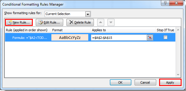
First, select your list of dates — for this example, select cells A2:A15. On the Home tab, click Conditional Formatting > Manage Rules. Refer to the screenshot below for guidance:

Once the Conditional Formatting Rules Manager dialog appears, click the New Rule button to create a custom formula-based rule.

In the New Formatting Rule dialog:
• Choose Use a formula to determine which cells to format. This option allows for flexible, date-driven highlighting.
• To highlight dates older than today, copy and paste the following formula into the Format values where this formula is true field:
=$A2<TODAY()• For highlighting dates that fall after today (i.e., upcoming future dates), use this formula:
=$A2>TODAY()• Next, click the Format button to define your preferred appearance (such as changing the fill color or font style). See example:
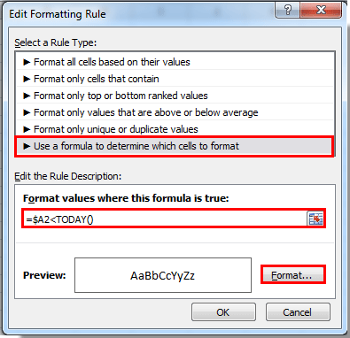
Specify your desired formatting in the Format Cells dialog (e.g., pick a color to make due dates or future dates stand out), then click OK.
Back in the Conditional Formatting Rules Manager, you’ll see your new rule listed. To activate the rule, click Apply. If you want to set up both due and future date highlighting, repeat steps to add a second rule using the other formula. When you return again to the Rules Manager, both rules will now appear.
After confirming with OK, your Excel sheet will now visually distinguish dates before and after today, offering clear indicators to prompt action or attention. Both overdue and upcoming date flags will automatically update as days change, so you always see the most relevant items at a glance.

Here’s the result: dates earlier or later than today are now highlighted per your format selection, simplifying review and follow-up.

Tips and Cautions: Ensure your date cells are formatted as dates (not text) for formulas to work correctly. If you experience unexpected results, double-check your date format. For very large datasets, conditional formatting can impact performance, so consider limiting the formatting range where possible.
Highlight dates before today or dates in the future with Kutools AI
For users seeking a simpler, smarter way to highlight overdue or future dates, Kutools AI for Excel streamlines the process. Rather than building conditional formatting rules manually, you can instruct Kutools AI directly in plain language. This method is ideal if you regularly need to highlight dates but want to save time or avoid formula setup, or if you work in environments where accuracy and efficiency are paramount.
To use Kutools AI for highlighting dates based on their relationship with today:
- Click "Kutools" > "AI Aide" to open the "Kutools AI Aide" pane, then do the following operations:
- Select the date range you wish to examine.
- In the AI Aide pane, type a command such as:
— For overdue dates: Highlight the dates before today with light blue color in the selected range
— For future dates: Highlight the dates after today with light blue color in the selected range - Press Enter or click Send. Kutools AI will analyze your request. Once processing is complete, click Execute to apply the formatting automatically.
Kutools AI automatically interprets your intent, choosing the appropriate formulas and formats, saving you time and minimizing manual setup errors. This approach is particularly useful in dynamic workbooks, for users less comfortable with formulas, or for those managing large, frequently updated date lists.
Caution: Kutools AI requires internet connectivity and up-to-date Kutools for Excel installation.
Flag and analyze dates with Excel helper column formulas
In many real-world cases, you might want more than color coding — for example, filtering, sorting, or counting records based on whether dates are before or after today. Using helper columns with Excel formulas allows you to flag such cases clearly and use other Excel features (like filters or PivotTables) for in-depth analysis.
Pros: Easy to set up, supports sorting/filtering, works in all Excel versions without special permissions. Cons: Requires additional space for helper columns; does not provide direct coloring unless combined with conditional formatting.
Here’s how to use a helper column for quick date analysis:
1. Insert a new column next to your date list (for example, column B next to your dates in A2:A15).
2. In cell B2 (assuming A2 is your first date), enter this formula to flag overdue dates:
=A2<TODAY()This formula will return TRUE if the date in A2 is before today and FALSE otherwise.
3. Alternatively, for highlighting future dates, use:
=A2>TODAY()4. Press Enter to confirm the formula, then drag the handle down to fill the column for all rows containing dates. The TRUE/FALSE results can now be used to sort or filter records by overdue or upcoming status.
If you prefer clear text labels, replace TRUE/FALSE with more descriptive flags. For example:
=IF(A2<TODAY(),"Overdue",IF(A2>TODAY(),"Upcoming","Today"))Copy this formula down to all relevant rows as needed. You can filter, sort or use the column as a criterion in other Excel features, such as Conditional Formatting or PivotTables. This approach is especially helpful for reports, dashboards, or preparing printable documents.
Note: If your date column is not column A, update the referenced cell in the formula accordingly. Ensure your data type for date cells is set to date, not text, to avoid inconsistent results.
Related articles:
- How to conditional format cells based on first letter/character in Excel?
- How to conditional format cells if containing #na in Excel?
- How to conditional format or highlight first recurrence in Excel?
- How to conditional format negative percentage in red in Excel?
Quick troubleshooting tips: If highlighting or formulas do not work as intended, always verify your date formatting and formula ranges. Use the Preview feature in Conditional Formatting to inspect which records are affected, and double-check for duplicate rules which may overlap or contradict each other. For larger tables, helper columns or VBA macros can streamline maintenance and save time when frequent updates are needed. Explore multiple methods to find the workflow best suited to your scenarios.
Best Office Productivity Tools
Supercharge Your Excel Skills with Kutools for Excel, and Experience Efficiency Like Never Before. Kutools for Excel Offers Over 300 Advanced Features to Boost Productivity and Save Time. Click Here to Get The Feature You Need The Most...
Office Tab Brings Tabbed interface to Office, and Make Your Work Much Easier
- Enable tabbed editing and reading in Word, Excel, PowerPoint, Publisher, Access, Visio and Project.
- Open and create multiple documents in new tabs of the same window, rather than in new windows.
- Increases your productivity by 50%, and reduces hundreds of mouse clicks for you every day!
All Kutools add-ins. One installer
Kutools for Office suite bundles add-ins for Excel, Word, Outlook & PowerPoint plus Office Tab Pro, which is ideal for teams working across Office apps.
- All-in-one suite — Excel, Word, Outlook & PowerPoint add-ins + Office Tab Pro
- One installer, one license — set up in minutes (MSI-ready)
- Works better together — streamlined productivity across Office apps
- 30-day full-featured trial — no registration, no credit card
- Best value — save vs buying individual add-in