How to COUNTIF filtered data/list with criteria in Excel?
You may notice that no matter whether you have filtered your table or not, the COUNTIF function will ignore the filtering and return a fixed value. In some cases, you are required to count filtered data with a specific criteria, so how to get it done? In this article, I will introduce a couple of ways to Countif filtered data/list in Excel quickly.
- Countif filtered data with criteria by adding a helper column in Excel
- Countif filtered data with criteria by Excel functions
- Countif filtered data with criteria by splitting data range into multiple sheets and then counting
Countif filtered data with criteria by adding a helper column in Excel
In this article, I will take the following table as an example. Here, I have filtered out Julie and Nicole in the Salesman column.
Original data:
Filtered data:
This method will guide you in adding an extra helper column, and then you can apply the COUNTIFS function to count the filtered data in Excel. (Note: This method requires you to filter your original table before following the steps below.)
1. Find a blank cell besides the original filtered table, say the cell G2, enter =IF(B2="Pear",1,""), and then drag the Fill Handle to the range you need. (Note: In the formula =IF(B2="Pear",1,""), B2 is the cell you will count, and the "Pear" is the criteria you will count by.)
Now a helper column is added besides original filtered table. The "1" indicates it's pear in the Column B, while blank hints it's not pear in Column B.
2. Find a blank cell and enter the formula =COUNTIFS(B2:B18,"Pear",G2:G18,"1"), and press the Enter key. (Note: In the formula =COUNTIFS(B2:B18,"Pear",G2:G18,"1"), the B2:B18 and G2:G18 are ranges you will count, and "Pear" and "1" are criteria you will count by.)
Now you will get the count number at once. Please note that the count number will not change if you disable filtering or change filtering.
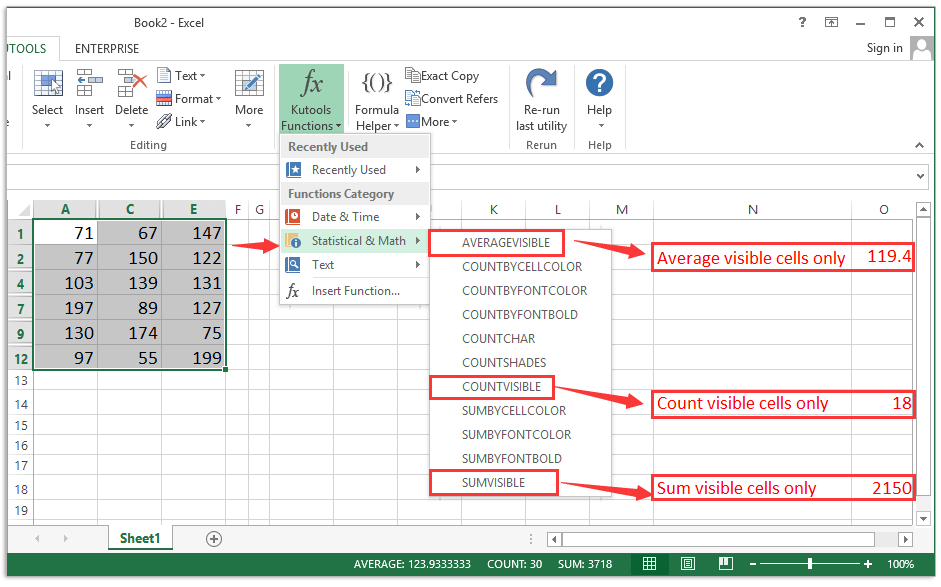
Sum/Count/Average visible cells only in a specified range with ignoring hidden or filtered cells/rows/columns
The normally SUM/Count/Average function will count all cells in the specified range on matter cells are hidden/filtered or not. While the Subtotal function can only sum/count/average with ignoring hidden rows. However, Kutools for Excel's SUMVISIBLE, COUNTVISIBLE, AVERAGEVISIBLE functions will easily calculate the specified range with ignoring any hidden cells, rows, or columns.
Kutools for Excel - Supercharge Excel with over 300 essential tools, making your work faster and easier, and take advantage of AI features for smarter data processing and productivity. Get It Now
Countif filtered data with criteria by Excel functions
If you want the count number changes as the filter changes, you can apply the SUMPRODUCT functions in Excel as following:
In a blank cell, enter the formula =SUMPRODUCT(SUBTOTAL(3,OFFSET(B2:B18,ROW(B2:B18)-MIN(ROW(B2:B18)),,1)),ISNUMBER(SEARCH("Pear",B2:B18))+0), and press the Enter key.

Notes:
(1) In the above formula, B2:B18 is the range you will count, and "Pear" is the criteria you will count by.
(2) The returning value will change when you disable filtering or filtering changes.
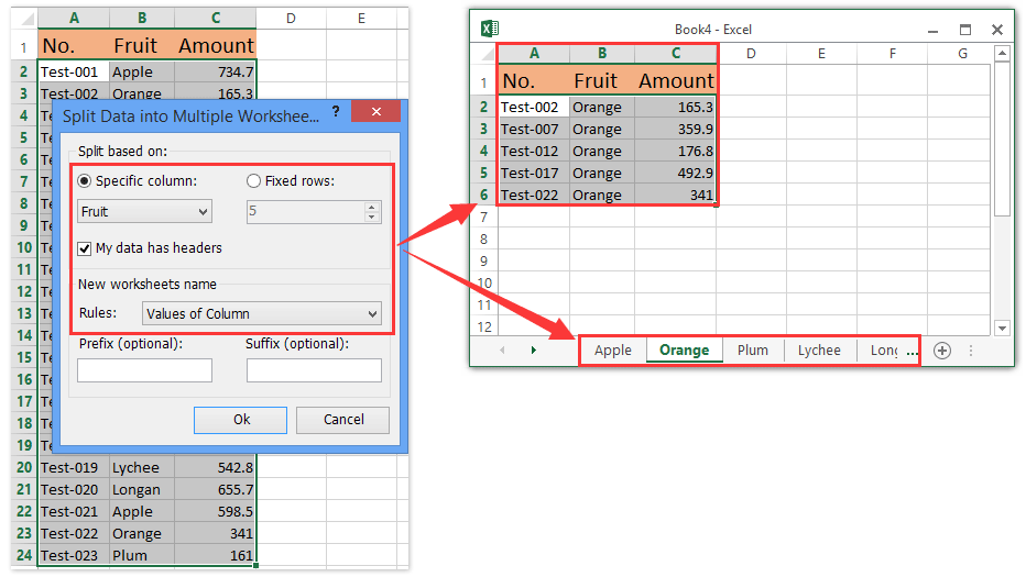
Easily split a range to multiple sheets based on criteria in a column in Excel
Comparing to complex array formulas, it may be much easier to save all filtered records into a new worksheet, and then apply the Count function to count the filtered data range or list.
Kutools for Excel’sSplit Data utility can help Excel users easily split a range to multiple worksheets based on criteria in one column of original range.
Kutools for Excel - Supercharge Excel with over 300 essential tools, making your work faster and easier, and take advantage of AI features for smarter data processing and productivity. Get It Now
Related Articles
How to count if cell does not contain text in Excel?
How to count if cells contain any date/data in Excel?
Best Office Productivity Tools
Supercharge Your Excel Skills with Kutools for Excel, and Experience Efficiency Like Never Before. Kutools for Excel Offers Over 300 Advanced Features to Boost Productivity and Save Time. Click Here to Get The Feature You Need The Most...
Office Tab Brings Tabbed interface to Office, and Make Your Work Much Easier
- Enable tabbed editing and reading in Word, Excel, PowerPoint, Publisher, Access, Visio and Project.
- Open and create multiple documents in new tabs of the same window, rather than in new windows.
- Increases your productivity by 50%, and reduces hundreds of mouse clicks for you every day!
All Kutools add-ins. One installer
Kutools for Office suite bundles add-ins for Excel, Word, Outlook & PowerPoint plus Office Tab Pro, which is ideal for teams working across Office apps.
- All-in-one suite — Excel, Word, Outlook & PowerPoint add-ins + Office Tab Pro
- One installer, one license — set up in minutes (MSI-ready)
- Works better together — streamlined productivity across Office apps
- 30-day full-featured trial — no registration, no credit card
- Best value — save vs buying individual add-in