Excel's IF function is a testament to the power and versatility of logical operations in data handling. The essence of the IF function is its ability to evaluate conditions and return specific outcomes based on those evaluations. It operates on a fundamental logic:

When combined with logical operators like AND, OR, and NOT, the IF function's capabilities significantly expand. The power of the combination lies in their ability to process multiple conditions simultaneously, providing results that can adapt to varied and complex scenarios. In this tutorial, we will explore how to effectively leverage these powerful functions in Excel to unlock new dimensions of data analysis and enhance your decision-making process. Let's dive in and discover the practical applications of these formidable Excel functions!

• IF AND formula (All Conditions True)
• IF OR formula (Any Condition True)
• IF NOT formula (Reverses Condition)

• If your condition is met, then calculate
• Case-sensitive AND, OR and NOT statements
• Integrating IF with nested AND, OR, NOT statements
• Nested IF functions with AND, OR, NOT

Amazing! Using Efficient Tabs in Excel Like Chrome, Edge, Firefox and Safari!
Save 50% of your time, and reduce thousands of mouse clicks for you every day!

IF AND formula

To assess multiple conditions and deliver a specific result when all conditions are met (TRUE), and a different result when any condition isn't met (FALSE), you can incorporate the AND function within the logical test of the IF statement. The structure for this is:

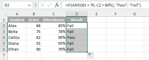
For instance, imagine you're a teacher analyzing student grades. You want to determine if a student passes based on two criteria: a score above 70 AND attendance over 80%.

1. Start by examining the first student's data, with their score in cell B2 and attendance in cell C2. For this student, apply the below formula in D2:

   =IF(AND(B2>70, C2>80%), "Pass", "Fail")

   Tip: This formula checks if the score in B2 is above 70 and attendance in C2 is over 80%. If both conditions are met, it returns "Pass"; otherwise, it returns "Fail".
2. Drag the formula down through the column to evaluate each student’s score and attendance.

   

IF OR Formula

To evaluate multiple conditions and return a specific result when any one of the conditions is met (TRUE), and a different result when none of the conditions are satisfied (FALSE), the OR function can be used within the logical test of the IF statement. The formula is structured as follows:

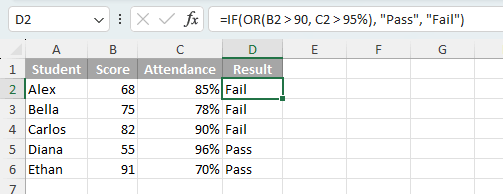
For example, in an educational context, consider a more flexible criterion for student passing. Here, a student is deemed to pass if they either score above 90 OR have an attendance rate higher than 95%.

1. Begin by evaluating the first student's performance, with their score in cell B2 and attendance in cell C2. Apply the formula in an adjacent cell, such as D2, to assess:

   =IF(OR(B2>90, C2>95%), "Pass", "Fail")

   Tip: This formula evaluates if the student either scores above 90 in B2 or has an attendance rate over 95% in C2. If either condition is met, it returns "Pass"; if not, "Fail".
2. Copy this formula down the column to apply it for each student in your list, enabling a quick assessment of each student’s eligibility for passing based on these criteria.

   

IF NOT Formula

To evaluate a condition and return a specific result if the condition is NOT met (FALSE), and a different result if the condition is met (TRUE), the NOT function within the IF statement is your solution. The structure for this formula is:

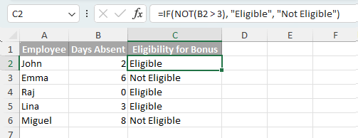
For a practical example, consider a workplace scenario where employee bonuses are determined based on their attendance record. Employees are eligible for a bonus if they have NOT been absent for more than 3 days.

1. To evaluate this for the first employee, whose days absent are in cell B2, use the formula:

   =IF(NOT(B2>3), "Eligible", "Not Eligible")

   Tip: This formula checks the number of days absent in B2. If it's NOT more than 3, it returns "Eligible"; otherwise, "Not Eligible".
2. Copy this formula down the column to apply it for each employee.

   

Advanced scenarios with IF and logical functions

In this section, we will explore the intricate use of Excel's IF function with logical operators like AND, OR, and NOT. This section covers everything from case-sensitive evaluations to nested IF statements, showcasing Excel's versatility in complex data analysis.

Amazing! Using Efficient Tabs in Excel Like Chrome, Edge, Firefox and Safari!
Save 50% of your time, and reduce thousands of mouse clicks for you every day!

If your condition is met, then calculate

In addition to providing predefined outcomes, the Excel IF function, when combined with logical operators like AND, OR, and NOT, can execute various calculations based on whether the set conditions are true or false. Here, we'll use the IF AND combination as an example to showcase this functionality.

Imagine you're managing a sales team and want to calculate bonuses. You decide that an employee receives a 10% bonus on their sales if they exceed $100 in sales AND have worked more than 30 hours in a week.

1. For the initial assessment, look at Alice’s data with her sales in cell B2 and hours worked in cell C2. Apply this formula in D2:

   =IF(AND(B2>100, C2>30), B2*0.1, 0)

   Tip: This formula calculates a 10% bonus on Alice’s sales if her sales exceed $100 and her hours worked are over 30. If both conditions are met, it calculates the bonus; otherwise, it returns 0.
2. Extend this formula to the rest of your team by copying it down the column. This approach ensures each employee’s bonus is calculated based on the same criteria.

   

Case-sensitive AND, OR and NOT statements

In Excel, while logical functions like AND, OR, and NOT are typically case-insensitive, there are scenarios where case sensitivity in text data is crucial. By integrating the EXACT function with these logical operators, you can effectively handle such case-sensitive conditions. In this section, we demonstrate the use of the IF and OR functions with a case-sensitive approach as an example.

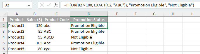
Imagine a retail scenario where a product is eligible for promotion if it either exceeds $100 in sales OR its code exactly matches "ABC" in a case-sensitive check.

1. For the first product listed in row 2, with its sales in cell B2 and product code in cell C2, use this formula in D2:

   =IF(OR(B2>100, EXACT(C2,"ABC")), "Promotion Eligible", "Not Eligible")

   Tip: This formula evaluates if the sales figure in B2 exceeds $100 or the product code in C2 is exactly "ABC". Meeting either of these conditions renders the product eligible for promotion; failing both makes it ineligible.
2. Replicate this formula across the column for all products to uniformly assess their eligibility for promotion based on sales and case-sensitive product code criteria.

   

Amazing! Using Efficient Tabs in Excel Like Chrome, Edge, Firefox and Safari!
Save 50% of your time, and reduce thousands of mouse clicks for you every day!

Integrating IF with nested AND, OR, NOT statements

Excel's IF function, when nested with AND, OR, and NOT, offers a streamlined approach to handle more layered conditions. This section provides an example showcasing the application of these nested functions in a retail setting.

Suppose you're overseeing a team responsible for various product categories, and you want to determine their bonus eligibility. An employee is eligible for a bonus if they: achieve sales over $100, AND either work more than 30 hours a week OR are NOT in the Electronics department.

1. First, assess Anne's performance, with her sales in cell B2, hours worked in cell C2, and department in cell D2. The formula in E2 would be:

   =IF(AND(B2>100, OR(C2>30, NOT(D2="Electronics"))), "Eligible", "Not Eligible")

   Tip: This formula checks if Anne has sales exceeding $100 and either works more than 30 hours or is not working with Electronics. If she meets these criteria, she is deemed "Eligible"; if not, "Not Eligible".
2. Copy this formula down the column for each employee to uniformly assess bonus eligibility, considering their sales, hours worked, and department.

   

Nested IF functions with AND, OR, NOT

When your data analysis involves multiple conditional checks, nested IF functions in Excel offer a powerful solution. This method entails constructing separate IF statements for distinct conditions, including AND, OR, and NOT logic, and then integrating them into one streamlined formula.

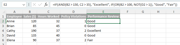
Consider a workplace where employee performance is rated as "Excellent", "Good", or "Fair" based on sales, hours worked, and policy adherence:

• "Excellent" for sales over $150 AND more than 35 hours worked.
• Otherwise, "Good" for sales above $100 OR policy violation NOT more than 1.
• "Fair" if neither of these conditions is met.

To assess each employee's performance according to the above conditions, please do as follows:

1. Begin with Anne's evaluation, whose sales are in cell B2, hours worked in cell C2, and policy violations in cell D2. The nested IF formula in E2 is:

   =IF(AND(B2>150, C2>35), "Excellent", IF(OR(B2>100, NOT(D2>1)), "Good", "Fair"))

   Tip: This formula first checks if Anne's sales and hours meet the criteria for "Excellent". If not, it evaluates whether she qualifies for "Good". If neither condition is met, she is categorized as "Fair".
2. Extend this nested IF formula to each employee to consistently assess their performance across multiple criteria.

   

Using IF with AND OR NOT: Frequently asked questions

This section aims to address frequently asked questions for using IF with AND, OR, and NOT in Microsoft Excel.

How many conditions can the AND, OR and NOT functions support?

• The AND and OR functions can support up to 255 individual conditions. However, it's advisable to use only a few to avoid overly complex formulas that are hard to maintain.
• The NOT function only takes one condition.

Can I use operators like <, >, = in these functions?

Certainly, in Excel's AND, OR, and NOT functions, you can utilize operators like less than (<), greater than (>), equals (=), greater than or equal to (>=), and more to establish conditions.

Why does a #VALUE error occur in these functions?

A #VALUE error in Excel's AND, OR, and NOT functions often arises if the formula doesn't meet any specified condition or if there's a problem with how the formula is structured. It indicates that Excel is unable to interpret the input or the conditions within the formula correctly.

Above is all the relevant content related to using IF with AND, OR and NOT functions in Excel. I hope you find the tutorial helpful. If you're looking to explore more Excel tips and tricks, please click here to access our extensive collection of over thousands of tutorials.