How to calculate average of dynamic range in Excel?

Formulas are a versatile approach for calculating the average of a dynamic range when the start or end point of your range changes frequently, as often happens with monthly sales or running totals. By letting an input cell determine the dynamic range boundary, you can quickly adapt to updated data without rewriting your formula.

To set this up, select a blank cell, such as Cell C4, and enter the following formula:

=IF(C2=0,"NA",AVERAGE(A2:INDEX(A:A,C2)))

Then press the Enter key to see the resulting average.

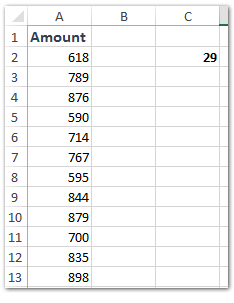
This formula automatically adjusts the range to include all cells from A2 to the row indicated by C2, so when C2's value changes, the averaged range changes as well. This makes it flexible for dynamically extending or contracting the averaging range as new data comes in or as you wish to analyze a specific subset.

Notes:

(1) In this formula =IF(C2=0,"NA",AVERAGE(A2:INDEX(A:A,C2))): A2 represents the first cell of the range to average, and C2 refers to the cell holding the row number of the last cell of the target range. Modify these references based on your own data structure as needed. Ensure that the C2 cell refers to a valid row, otherwise you'll get unexpected results or "NA".

(2) As an alternative, you can use:

=AVERAGE(INDIRECT("A2:A"&C2))

This method is equally effective as it creates a text reference for the range, which INDIRECT then interprets dynamically. However, be cautious when using INDIRECT with closed workbooks or large datasets, as it may impact calculation speed and is not as efficient as INDEX for volatile data.

Practical Tip: When your data continuously grows (such as appending new rows every day), you can use a COUNTA or COUNT function to automatically set the upper bound cell reference—this ensures your dynamic range always covers up-to-date entries.

Applicable scenarios: Daily data logs, time series entries, or any analysis where the start or end of the range is guided by user input or a summary cell. Advantages: Direct, does not require additional tools. Limitation: Needs manual formula adjustment if row locations change drastically.

For situations where your dynamic range is defined not by position but by specific criteria (such as a region, category, or user-defined label), you can combine dynamic named ranges and functions like INDIRECT to adapt your calculations. This is especially helpful for dashboards where users select from a dropdown and instantly see related averages.

First, group your dataset by heading rows or columns. Here’s how:

1. Select the entire area (such as A1:D11), and click the Create names from selection button in the Name manager pane. In the popup dialog, check both Top row and Left column options, then click OK. This step assigns named ranges to data in rows and columns automatically, which simplifies referencing in formulas.

2. In your chosen blank cell, input this formula:

=AVERAGE(INDIRECT(G2))

Here, G2 is the criteria cell where users type or select the row or column header name. When G2 changes (e.g., from "Region1" to "Region2"), the formula dynamically calculates the average for the corresponding range. Always ensure the inputs in G2 exactly match the defined names (including case sensitivity) to avoid #REF! errors.

Best for: Reporting dashboards, criteria-driven analytics. Advantages: Enables very flexible dynamic reporting or single-cell analysis by user interaction. Limitation: Relies on proper name management and consistent input values.

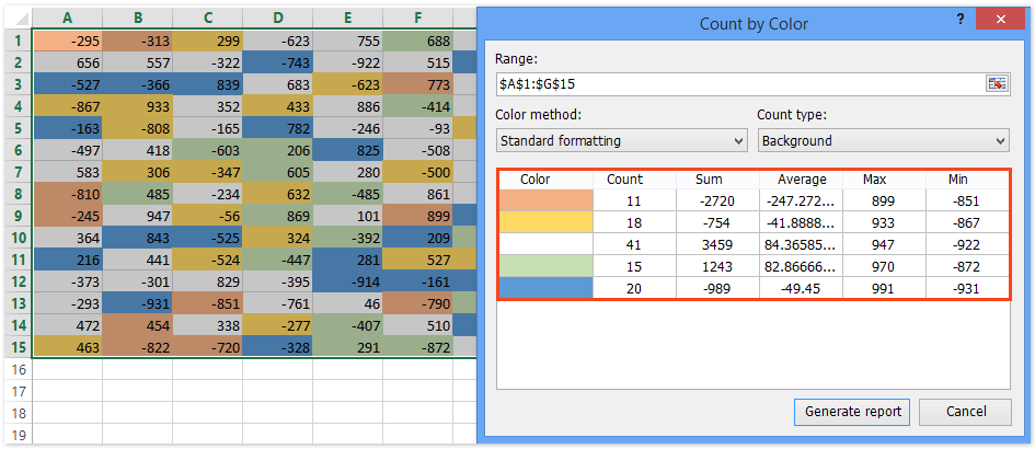
Automatically Count/Sum/Average cells by fill color in Excel

Sometimes you mark cells by fill color, and then count/sum up these cells or calculate these cells’ average later. Kutools for Excel’s Count by Color utility can help you solve it with ease.

For advanced dynamic behaviors, such as averaging the last N rows, averaging based on multiple dynamic criteria, or even combining data across multiple sheets, you can create a custom VBA macro. This method is particularly helpful when built-in formulas become too complex for your scenario, or when you need automation that adapts to frequently changing structures.

For example, you may want to calculate the average of the last N rows in column A, where N is typed by the user, or average values from non-contiguous, user-specified ranges.

1. Go to Developer Tools > Visual Basic to open the Microsoft Visual Basic for Applications editor. Then select Insert > Module and paste in the following VBA code:

Sub DynamicAverage_LastNRows()
    Dim ws As Worksheet
    Dim rng As Range
    Dim lastRow As Long
    Dim N As Long
    Dim result As Double
    Dim xTitleId As String
    
    On Error Resume Next
    xTitleId = "KutoolsforExcel"
    
    Set ws = Application.ActiveSheet
    lastRow = ws.Cells(ws.Rows.Count, "A").End(xlUp).Row
    N = Application.InputBox("How many last rows to average?", xTitleId, 5, Type:=1)
    
    If N <= 0 Or N > lastRow - 1 Then
        MsgBox "Invalid input for N!", vbExclamation
        Exit Sub
    End If
    
    Set rng = ws.Range("A" & lastRow - N + 1, "A" & lastRow)
    result = Application.WorksheetFunction.Average(rng)
    
    MsgBox "Average of the last " & N & " rows in column A: " & result, vbInformation
End Sub

2. Click the button to run the macro. In the pop-up dialog, input the number of last rows you want to average (such as 5,10, etc.) and press OK. The result will appear in a message box.

To average with more complex conditions (e.g., based on criteria or from multiple sheets), you can adapt the VBA code accordingly—for example, by adding InputBoxes for a criteria value, or looping through several worksheets to combine ranges before averaging.

This approach offers maximum flexibility and can automate complex or repetitive dynamic average calculations. However, ensure you enable macros and use this method in a trusted workbook to avoid security risks. Save your work before running new macros, and consider creating backups when automating changes.

Pros: Allows automation, handles complex or large data scenarios, can be tailored for very specific business logic. Cons: Requires a basic understanding of VBA, and procedures need to be maintained if structure changes.