How to vlookup return value in adjacent or next cell in Excel?
How can we vlookup a value but to find the value in adjacent or next cell? In this article, we will guide you through how to vlookup a value and return value in adjacent or next cell in Excel.
Vlookup return value in adjacent cell with formula in Excel
Easily vlookup return value in adjacent cell with Kutools for Excel
Vlookup return value in the next cell in Excel
Vlookup return value in adjacent cell in Excel
For example, you have two columns as shown in following screenshot. To vlookup the largest weight in column A and return the adjacent cell value of column B, please do as follows.

1. Select a blank cell (here I select cell C3), enter the below formula into it, and then press the Enter key.
=VLOOKUP(MAX(A2:A11), A2:B11, 2, FALSE)

Then the adjacent cell value of the largest weight in column A is populated in the selected cell.
Besides, you can vlookup and get the adjacent cell value based on a cell reference.
For example, the referenced cell is C2 which locates value 365, for vlookup this value and return the value in adjacent cell. You just need to change the above formula to below, and then press the Enter key. See screenshot:
=VLOOKUP(C2, A2:B11, 2, FALSE)

This Index function also works: =INDEX($B$1:$B$7, SMALL(IF(ISNUMBER(SEARCH($C$2, $A$1:$A$7)), MATCH(ROW($A$1:$A$7), ROW($A$1:$A$7))), ROW(A1))) + Ctrl + Shift + Enter.
Vlookup return value in the next cell in Excel
Besides returning value in an adjacent cell, you can vlookup and return value in the next cell of the adjacent cell in Excel. See screenshot:

1. Select a blank cell, enter the below formula into it, and then press the Enter key.
=INDEX(B2:B7,MATCH(680,A2:A7,0)+1)

Then you can see the value in next cell is populated into the selected cell.
Note: 680 in the formula is the value which I vlookup in this case, you can change it as you want.
Easily vlookup return value in adjacent cell with Kutools for Excel
With the Look for a value in list utility of Kutools for Excel, you can vlookup and return value in adjacent cell without formulas.
Before applying Kutools for Excel, please download and install it firstly.
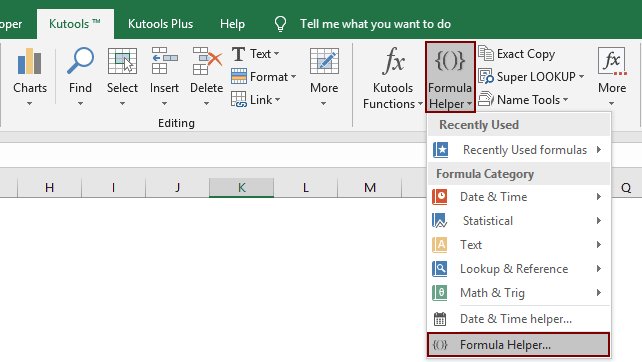
1. Select a blank cell for locating the adjacent cell value. Then click Kutools > Formula Helper > Formula Helper.
3. In the Formulas Helper dialog box, please configure as follows:
- 3.1 In the Choose a formula box, find and select Look for a value in list;
Tips: You can check the Filter box, enter certain word into the text box to filter the formula quickly. - 3.2 In the Table_array box, select the range contains the vlookup value and the adjacent value you will return (in this case, we select range A2:C10);
- 3.2 In the Lookup_value box, select the cell you will return the value based on (In this case, we select cell E2);
- 3.3 In the Column box, specify the column you will return the matched value from. Or you can enter the column number into the textbox directly as you need.
- 3.4 Click the OK button. See screenshot:

Then you will get the adjacent cell value of cell A8.

If you want to have a free trial (30-day) of this utility, please click to download it, and then go to apply the operation according above steps.
Easily vlookup return value in adjacent cell with Kutools for Excel
Best Office Productivity Tools
Supercharge Your Excel Skills with Kutools for Excel, and Experience Efficiency Like Never Before. Kutools for Excel Offers Over 300 Advanced Features to Boost Productivity and Save Time. Click Here to Get The Feature You Need The Most...
")
Office Tab Brings Tabbed interface to Office, and Make Your Work Much Easier
- Enable tabbed editing and reading in Word, Excel, PowerPoint, Publisher, Access, Visio and Project.
- Open and create multiple documents in new tabs of the same window, rather than in new windows.
- Increases your productivity by 50%, and reduces hundreds of mouse clicks for you every day!
")