How to vlookup to return multiple values in a single cell in Excel?
VLOOKUP is a powerful function in Excel, but by default, it only returns the first matching value. What if you need to retrieve all matching values and combine them into one cell? This is a common requirement when analyzing datasets or summarizing information. In this guide, we’ll walk you through step-by-step methods to return multiple values into a single cell using both formulas and helpful feature.
Return multiple values into one cell with TEXTJOIN function (Excel 2019 and Office 365)
Return multiple values into one cell by Kutools
Return multiple values into one cell with User Defined Function
Return multiple values into one cell with TEXTJOIN function (Excel 2019 and Office 365)
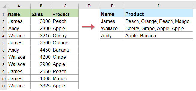
If you have the higher version of the Excel such as Excel 2019 and Office 365, there is a new function - TEXTJOIN, with this powerful function, you can quickly vlookup and return all matching values into one cell.
Return all matching values into one cell
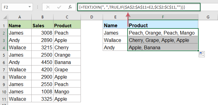
Please apply the below formula into a blank cell where you want to put the result, then press Ctrl + Shift + Enter keys together to get the first result, and then drag the fill handle down to the cell you want to use this formula, and you will get all corresponding values as below screenshot shown:
Return all matching values without duplicates into one cell
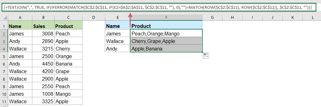
If you want to return all matching values based on the lookup data without duplicates, the below formula may help you.
Please copy and paste the following formula into a blank cell, then press Ctrl + Shift + Enter keys together to get the first result, and then copy this formula to fill other cells, and you will get all corresponding values without the dulpicate ones as below screenshot shown:
Return multiple values into one cell by Kutools
With Kutools for Excel's "Advanced Combine Rows" feature, you can easily retrieve multiple matching values into a single cell—no complex formulas required! Say goodbye to manual workarounds and unlock a more efficient way to handle your lookup tasks in Excel. Let’s explore how Kutools for Excel makes it all possible!
After installing Kutools for Excel, please do as follows:
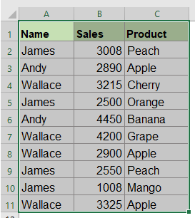
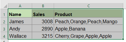
1. Select the data range that you want to combine one column data based on another column.
2. Click "Kutools" > "Merge & Split" >" Advanced Combine Rows", see screenshot:

3. In the popped out "Advanced Combine Rows" dialog box:
- Click the key column name to be combined based on, and then click "Primary Key".
- Then click another column that you want to combine its data based on the key column, and click the drop down list from the "Operation" field,choose one separator for separating the combined data from the "Combine" section.
- Then, click OK button.

All corresponding values from another column, based on the same value, are combined into a single cell. See screenshots:
 |  |
Tips: If you want to remove duplicate content while merging cells, simply check the "Delete Duplicate Values" option in the dialog box. This ensures that only unique entries are combined into a single cell, making your data cleaner and more organized without any extra effort. See screenshots:
 |  |
Download and free trial Kutools for Excel Now !
Return multiple values into one cell with User Defined Function
The above TEXTJOIN function is only available for Excel 2019 and Office 365, if you have other lower Excel versions, you should use some codes for finishing this task.
Return all matching values into one cell
1. Hold down the "ALT + F11" keys, and it opens the "Microsoft Visual Basic for Applications" window.
2. Click "Insert" > "Module", and paste the following code in the Module Window.
VBA code: Vlookup to return multiple values into one cell
Function ConcatenateIf(CriteriaRange As Range, Condition As Variant, ConcatenateRange As Range, Optional Separator As String = ",") As Variant
'Updateby Extendoffice
Dim xResult As String
On Error Resume Next
If CriteriaRange.Count <> ConcatenateRange.Count Then
    ConcatenateIf = CVErr(xlErrRef)
    Exit Function
End If
For i = 1 To CriteriaRange.Count
    If CriteriaRange.Cells(i).Value = Condition Then
        xResult = xResult & Separator & ConcatenateRange.Cells(i).Value
    End If
Next i
If xResult <> "" Then
    xResult = VBA.Mid(xResult, VBA.Len(Separator) + 1)
End If
ConcatenateIf = xResult
Exit Function
End Function
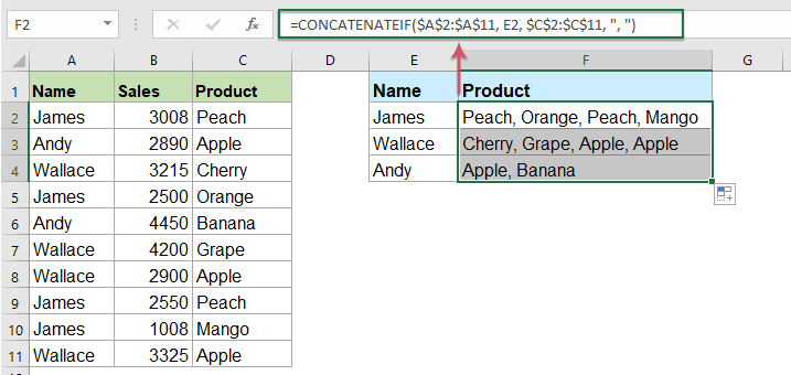
3. Then save and close this code, go back to the worksheet, and enter this formula: =CONCATENATEIF($A$2:$A$11, E2, $C$2:$C$11, ", ") into a specific blank cell where you want to place the result, then drag the fill handle down to get all the corresponding values in one cell that you want, see screenshot:
Return all matching values without duplicates into one cell
To ignore the duplicates in the returned matching values, please do with the below code.
1. Hold down the "Alt + F11" keys to open the "Microsoft Visual Basic for Applications" window.
2. Click "Insert" > "Module", and paste the following code in the Module Window.
VBA code: Vlookup and return multiple unique matched values into one cell
Function MultipleLookupNoRept(Lookupvalue As String, LookupRange As Range, ColumnNumber As Integer)
'Updateby Extendoffice
    Dim xDic As New Dictionary
    Dim xRows As Long
    Dim xStr As String
    Dim i As Long
    On Error Resume Next
    xRows = LookupRange.Rows.Count
    For i = 1 To xRows
        If LookupRange.Columns(1).Cells(i).Value = Lookupvalue Then
            xDic.Add LookupRange.Columns(ColumnNumber).Cells(i).Value, ""
        End If
    Next
    xStr = ""
    MultipleLookupNoRept = xStr
    If xDic.Count > 0 Then
        For i = 0 To xDic.Count - 1
            xStr = xStr & xDic.Keys(i) & ","
        Next
        MultipleLookupNoRept = Left(xStr, Len(xStr) - 1)
    End If
End Function
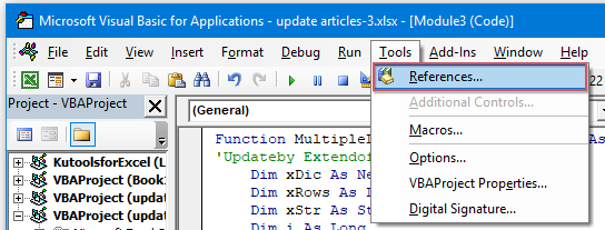
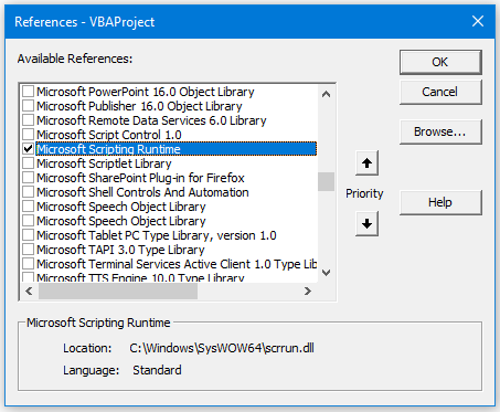
3. After inserting the code, then click "Tools" > "References" in the opened "Microsoft Visual Basic for Applications" window, and then, in the popped out "References – VBAProject" dialog box, check "Microsoft Scripting Runtime" option in the "Available References" list box, see screenshots:
 |  |
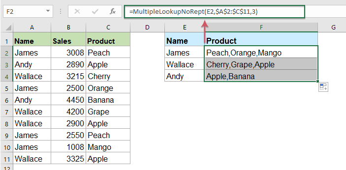
4. Then click OK to close the dialog box, save and close the code window, return to the worksheet, and enter this formula: =MultipleLookupNoRept(E2,$A$2:$C$11,3) into a blank cell where you want to output the result, and then drag the fill hanlde down to get all matching values, see screenshot:
Whether you opt for formulas like TEXTJOIN combined with array functions, leverage tools like Kutools for Excel or User Defined function, all approaches help simplify complex lookup tasks. Choose the method that best suits your needs. If you're interested in exploring more Excel tips and tricks, our website offers thousands of tutorials.
More relative articles:
- VLOOKUP Function With Some Basic And Advanced Examples
- In Excel, the VLOOKUP function is a powerful function for most of Excel users, which is used to look for a value in the leftmost of the data range, and return a matching value in the same row from a column you specified. This tutorial is talking about how to use the VLOOKUP function with some basic and advanced examples in Excel.
- Return multiple matching values based on one or multiple criteria
- Normally, lookup a specific value and return the matching item is easy for most of us by using the VLOOKUP function. But, have you ever tried to return multiple matching values based on one or more criteria? In this article, I will introduce some formulas for solving this complex task in Excel.
- Vlookup And Return Multiple Values Vertically
- Normally, you can use the Vlookup function to get the first corresponding value, but, sometimes, you want to return all matching records based on a specific criterion. This article, I will talk about how to vlookup and return all matching values vertically, horizontally or into one single cell.
- Vlookup And Return Multiple Values From Drop Down List
- In Excel, how could you vlookup and return multiple corresponding values from a drop down list, which means when you choose one item from the drop down list, all of its relative values are displayed at once. This article, I will introduce the solution step by step.
Best Office Productivity Tools
Supercharge Your Excel Skills with Kutools for Excel, and Experience Efficiency Like Never Before. Kutools for Excel Offers Over 300 Advanced Features to Boost Productivity and Save Time. Click Here to Get The Feature You Need The Most...
Office Tab Brings Tabbed interface to Office, and Make Your Work Much Easier
- Enable tabbed editing and reading in Word, Excel, PowerPoint, Publisher, Access, Visio and Project.
- Open and create multiple documents in new tabs of the same window, rather than in new windows.
- Increases your productivity by 50%, and reduces hundreds of mouse clicks for you every day!
All Kutools add-ins. One installer
Kutools for Office suite bundles add-ins for Excel, Word, Outlook & PowerPoint plus Office Tab Pro, which is ideal for teams working across Office apps.
- All-in-one suite — Excel, Word, Outlook & PowerPoint add-ins + Office Tab Pro
- One installer, one license — set up in minutes (MSI-ready)
- Works better together — streamlined productivity across Office apps
- 30-day full-featured trial — no registration, no credit card
- Best value — save vs buying individual add-in