How to count unique values based on another column in Excel?

When working with data in Excel, you might encounter situations where you need to count the number of unique values in one column, grouped by the values in another column. For example, I have two columns data, now, I need count the unique names in column B based on the content of column A as left screenshot shown. This article provides a detailed guide on how to achieve this efficiently, along with optimization tips to enhance performance and accuracy.
Count unique values based on another column
Count unique values based on another column with a formula
If you prefer using formulas, you can use a combination of SUMPRODUCT and COUNTIF functions to count unique values.
1. Enter the following formula into a blank cell where you want to put the result, then drag the fill handle down to get the unique values of the corresponding criteria. See screenshot:
=SUMPRODUCT(($A$2:$A$18=D2)/COUNTIF($B$2:$B$18,$B$2:$B$18&""))
- A2:A18=D3: This part checks if the course in column A is the cell value D3, returning an array of TRUE/FALSE values.
- COUNTIF(B2:B18,B2:B18&""): This counts the occurrences of each student name in column B.
- SUMPRODUCT: This function sums the results of the division, effectively counting unique names.
Count unique values based on another column with Kutools for Excel
Streamline your data analysis with Kutools for Excel, a powerful add-in that simplifies complex tasks. If you need to count unique values based on another column, Kutools offers an intuitive and efficient solution.
After installing Kutools for Excel, please click "Kutools" > "Merge & Split" > "Advanced Combine Rows" to go to the "Advanced Combine Rows" dialog box.
In the "Advanced Combine Rows" dialog box, please set the following operations:
- Click the column name that you want to base your unique count on, here, I will click Course, and then select "Primary Key" from the drop-down list in the "Operation" column;
- Then, select the column name you want to count the values, and then select "Count" from the drop-down list in the "Operation" column;
- Check "Delete duplicate values" option to count only the unique values;
- At last, click OK Button.
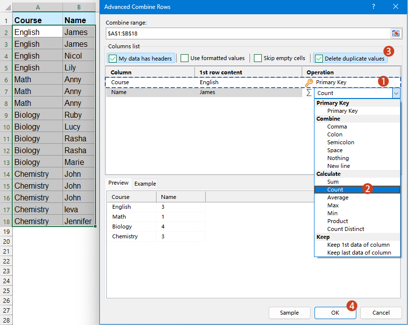
Result: Kutools will generate a table with the unique counts based on your specified column.
Count unique values based on another column with UNIQUE and FILTER functions
Excel 365 or Excel 2021 and later versions introduces powerful dynamic array functions like UNIQUE and FILTER, which make it easier than ever to count unique values based on another column.
Enter or copy the below formula into a blank cell to put the result, and then drag the formula down to fill it the other cells, see screenshot:
=IFERROR(ROWS(UNIQUE(FILTER($B$2:$B$18,$A$2:$A$18=D2))), 0)
- FILTER($B$2:$B$18, $A$2:$A$18=D2): Filters the values in column B where the corresponding value in column A matches the value in D2.
- UNIQUE(...): Removes duplicates from the filtered list, keeping only unique values.
- ROWS(...): Counts the number of rows in the unique list, effectively giving the count of unique values.
- IFERROR(..., 0): If there’s an error (e.g., no matching values in column A), the formula returns 0 instead of an error.
In summary, counting unique values based on another column in Excel can be achieved through various methods, each suited to different versions and user preferences. By choosing the method that best fits your Excel version and workflow, you can efficiently manage and analyze your data with precision and ease. If you're interested in exploring more Excel tips and tricks, our website offers thousands of tutorials.
Related articles:
How to count the number of unique values in a range in Excel?
How to count unique values in a filtered column in Excel?
How to count same or duplicate values only once in a column?
Best Office Productivity Tools
Supercharge Your Excel Skills with Kutools for Excel, and Experience Efficiency Like Never Before. Kutools for Excel Offers Over 300 Advanced Features to Boost Productivity and Save Time. Click Here to Get The Feature You Need The Most...
Office Tab Brings Tabbed interface to Office, and Make Your Work Much Easier
- Enable tabbed editing and reading in Word, Excel, PowerPoint, Publisher, Access, Visio and Project.
- Open and create multiple documents in new tabs of the same window, rather than in new windows.
- Increases your productivity by 50%, and reduces hundreds of mouse clicks for you every day!
All Kutools add-ins. One installer
Kutools for Office suite bundles add-ins for Excel, Word, Outlook & PowerPoint plus Office Tab Pro, which is ideal for teams working across Office apps.
- All-in-one suite — Excel, Word, Outlook & PowerPoint add-ins + Office Tab Pro
- One installer, one license — set up in minutes (MSI-ready)
- Works better together — streamlined productivity across Office apps
- 30-day full-featured trial — no registration, no credit card
- Best value — save vs buying individual add-in