How to vlookup to compare two lists in separated worksheets?

Vlookup to compare two lists in separate worksheets with formulas

One practical and direct approach to compare lists situated in different Excel worksheets is by utilizing the VLOOKUP function. This method helps you efficiently extract or flag all names found in both Names-1 and Names-2:

1. In the Names-1 sheet, choose a cell adjacent to your list data (for instance, cell B2) and enter the following formula:

=VLOOKUP(A2,'Names-2'!$A$2:$A$19,1,FALSE)

Then press Enter. If the name in the current row exists in Names-2, the formula returns the name; if not, a #N/A error will be displayed. See the example below:

2. Copy the formula down by dragging the fill handle to compare each name in Names-1 against all names in Names-2. Matching entries will show the name, while those not found will display an error value:

Notes:

1. For more clarity, you might use this alternative formula to return "Yes" or "No" indicators for matches:

=IF(ISNA(VLOOKUP(A2,'Names-2'!$A$2:$A$19,1,FALSE)), "No", "Yes")

This formula displays "Yes" for names present in both sheets and "No" for names only found in Names-1:

2. When using these formulas, replace A2 with the first cell in your list, Names-2 with the name of the reference sheet, and adjust $A$2:$A$19 to match the actual data range in your worksheet. Remember, ranges must start and end with the correct row numbers to ensure all your data is included.

3. Tips for use: If you encounter #N/A errors where there should be matches, check carefully for possible issues caused by extra spaces, data formatting differences (text vs. number), or typos in your lists. Use TRIM or CLEAN in a helper column to clean up data if needed.

4. To avoid accidental overwrites, consider backing up your data before applying bulk formulas. Additionally, after the comparison, you can use Filter on your formula result column to quickly view all matches or unique items.

Vlookup to compare two lists in separate worksheets with Kutools for Excel

If you have Kutools for Excel, its Select Same & Different Cells feature can help you rapidly compare two lists from different worksheets and select or highlight common names between these two sheets—all without entering complex formulas. This method is especially effective when you’re dealing with large volumes of data or want a visual, color-coded result that’s easy to interpret at a glance.

After installing Kutools for Excel, follow these steps to easily compare your lists:

1. Go to the Kutools tab, then click Select > Select Same & Different Cells as shown below:

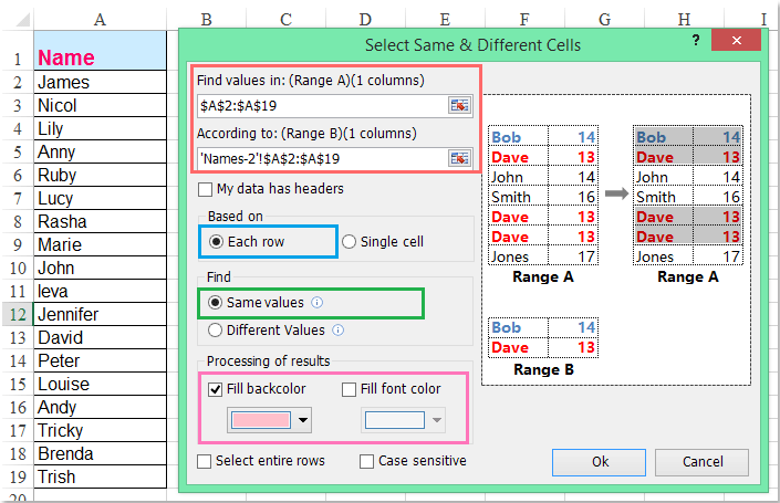
2. In the opened Select Same & Different Cells dialog box:

(1.) Under Find values in, select the range from Names-1 you need to compare;

(2.) Under According to, select the range from Names-2 to compare against;

(3.) In the Based on section, choose Each row to compare rows respectively;

(4.) From the Find section, select Same Values to identify and highlight matching names;

(5.) Optionally, you can set a background or font color to highlight the results and make matches stand out visually.

3. Click Ok, and you will see a prompt box showing how many matching cells have been found and highlighted. All names present in both lists will be selected and visually emphasized, simplifying further review or modification:

Click to Download and free trial Kutools for Excel Now !

Practical Tips: If your worksheets contain large datasets, consider using the filter function after highlighting to quickly review only the matches. Also, before running the comparison, double-check that your range selections correctly align and do not include header rows unless intended, as mismatches can affect results.

In rare cases, if the function does not return expected results, check if both lists are formatted the same way (for example, both as text, with no hidden leading/trailing spaces), as formatting discrepancies might cause matches to be missed.

Conditional Formatting with Formula Across Sheets

If you prefer not to write formulas in columns or use add-ins, you can utilize Conditional Formatting with a custom formula to visually identify matching names in one sheet based on another sheet’s data. This method is straightforward and requires no VBA, but does not return a separate list of results—rather, it simply formats matches for quick at-a-glance review.

Applicable Scenarios: This solution is ideal for users who want a non-intrusive, visual indicator of matching values and do not wish to alter worksheet structure. The limitation is that Conditional Formatting rules cannot directly reference another workbook, and formula cross-sheet referencing works only within the same file.

Steps:

1. In Names-1, select the range to which you wish to apply highlighting (for example, A2:A19).

2. Go to Home > Conditional Formatting > New Rule > Use a formula to determine which cells to format.

3. In the formula box, enter the following formula:

=COUNTIF('Names-2'!$A$2:$A$19,A2)>0

This checks if the value in A2 of Names-1 exists anywhere in Names-2!A2:A19.

4. Click Format to choose a highlight color, then click OK to apply the rule. Any matches will be highlighted automatically in your selected range.

Practical Tips: You can adjust the ranges based on your actual data, and the COUNTIF step can be combined with filtering to focus on only highlighted cells. Make sure both worksheets are within the same workbook when setting up cross-sheet references, as Excel does not support conditional formatting rules referencing external files.

Error Reminders: If highlights do not appear as expected, check your cell range selections and cross-sheet references for errors. Ensure there are no leading/trailing spaces or format inconsistencies causing missed matches. If necessary, use TRIM in a helper column to clean up the lists for accurate comparison.

VBA Code - Automatically compare lists and highlight or extract matches

For users who are comfortable with macros, using VBA code provides a highly flexible and automated way to compare two lists in separate worksheets. This approach allows you to highlight matching names or extract the matching values to a new location, which can be especially useful when handling large volumes of data or needing quick updates as your lists change.

Applicable Scenarios: This solution is particularly effective when you wish to repeatedly run comparisons, handle very large datasets, automate reporting, or further customize how matches are processed or presented. While knowledge of VBA is needed, you gain the benefit of full automation and control. A downside is that macros must be enabled in the workbook, which may not be permitted in all environments due to security settings.

How to run the macro to highlight matches in Names-1 if present in Names-2:

1. Click Developer Tools > Visual Basic to launch the Microsoft Visual Basic for Applications window. In the window, click Insert > Module and paste the following code into the new module:

Sub HighlightMatchingNames()
    Dim ws1 As Worksheet
    Dim ws2 As Worksheet
    Dim rng1 As Range
    Dim cell As Range
    Dim matchFound As Range
    
    On Error Resume Next
    xTitleId = "KutoolsforExcel"
    
    Set ws1 = Worksheets("Names-1")
    Set ws2 = Worksheets("Names-2")
    
    Set rng1 = ws1.Range("A2", ws1.Cells(ws1.Rows.Count, "A").End(xlUp))
    
    ws1.Range("A2:A" & ws1.Cells(ws1.Rows.Count, "A").End(xlUp).Row).Interior.ColorIndex = xlNone
    
    For Each cell In rng1
        Set matchFound = ws2.Range("A2:A" & ws2.Cells(ws2.Rows.Count, "A").End(xlUp).Row).Find( _
            What:=cell.Value, LookIn:=xlValues, LookAt:=xlWhole)
        
        If Not matchFound Is Nothing And cell.Value <> "" Then
            cell.Interior.Color = vbYellow
        End If
    Next cell
End Sub

2. In the VBA editor, click the button to run the code. This macro will scan the names in column A of the "Names-1" worksheet, and if a name also appears in column A of the "Names-2" worksheet, it will highlight that cell in "Names-1" with yellow fill color. Any previous highlights in the range will be cleared before the new comparison.

Troubleshooting: If no cells are highlighted, check that both worksheets are named exactly "Names-1" and "Names-2", and that your data ranges start from A2. Ensure macros are enabled, and that neither worksheet is protected or filtered. This approach can be easily customized; for example, you can change the highlight color, or adapt the code to copy matched results to another sheet or column.

Summary and Suggestions: Depending on your needs and technical comfort level, you can choose from built-in formula solutions, macro automation, smart add-ins like Kutools, or straightforward visualization with Conditional Formatting. When using formulas or VBA, always review your data for extra spaces or inconsistent formatting, which are common sources of errors. Back up your data before making batch changes, especially when using macros or add-ins for the first time. If you encounter issues such as formulas not updating or incorrect matches, check for relative/absolute range mistakes and verify worksheet names. By selecting the method that matches your workflow, you can effectively and efficiently compare lists across different sheets in Excel.