How to compare two columns and return values from the third column in Excel?
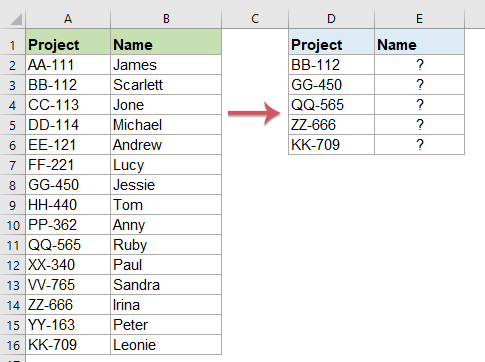
For example, I have the following two columns, column A is some projects, and column B is the corresponding names. And here, I have some random projects in column D, now, I want to return the corresponding names from column B based on the projects in column D. How can you compare columns A and D and return the corresponding values from column B in Excel?
Compare two columns and return value from third column with VLOOKUP function
Compare two columns and return value from third column with INDEX and MATCH functions
Vlookup multiple columns and return the corresponding values with INDEX and MATCH functions
Using Kutools for Excel to compare two columns and return value form third column
Compare two columns and return value from third column with VLOOKUP function
The VLOOKUP function can help you to compare two columns and extract the corresponding values from the third column, please do as follows:
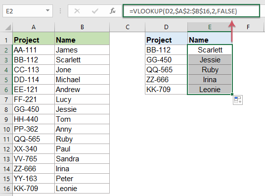
1. Enter any of the below two formulas into a blank cell besides the compared column, E2 for this instance:
=VLOOKUP(D2,$A$2:$B$16,2,FALSE)=IFERROR(VLOOKUP(D2,$A$2:$B$16,2,FALSE), "")2. Then press "Enter" key to get the first corresponding value, and then select the formula cell and drag the fill handle down to the cells that you want to apply this formula, and all the corresponding values have been returned at once, see screenshot:
Compare two columns and return value from third column with INDEX and MATCH functions
In Excel, the INDEX and MATCH functions also can help you to solve this task, please do as follows:
1. Enter any of the below two formulas into a blank cell where you want to return the result:
=INDEX($B$2:$B$16, MATCH(D2,$A$2:$A$16,0))=IFERROR(INDEX($B$2:$B$16, MATCH(D2,$A$2:$A$16,0)), "")2. Then press "Enter" key to get the first corresponding value, and then select the formula cell and copy to the rest cells you need, and all the corresponding values have been returned, see screenshot:

If you often use the VLOOKUP function in Excel, Kutools for Excel's "Super LOOKUP" provides powerful VLOOKUP formulas, allowing you to perform lookups without needing to remember complex formulas.

Kutools for Excel - Supercharge Excel with over 300 essential tools, making your work faster and easier, and take advantage of AI features for smarter data processing and productivity. Get It Now
Vlookup multiple columns and return the corresponding values with INDEX and MATCH functions
Sometimes, you may have a range of data which contains three columns, now you want to lookup on the table to match two criteria values, if both the two values matches, it will return the data from the third column C.

To dea with this job, please apply the following formula:
=INDEX($C$2:$C$16,MATCH(E2&F2, $A$2:$A$16&$B$2:$B$16,0))Then press "Ctrl" + "Shift" + "Enter" keys together to get the first result, see screenshot

Copy and paste this array formula into other cells to get the complete results:

Using Kutools for Excel to compare two columns and return value form third column
Kutools for Excel’s "Look for a value in list" also can help you to return the corresponding data from another data range.
1. Click a cell where you want to put the matched result.
2. Then click "Kutools" > "Formula Helper" > "Formula Helper", see screenshot:

3. In the "Formulas Helper" dialog box, please do the following operations:
- In the "Formula Type" drop down list, please select "Lookup" option;
- Then, select "Look for a value in list" option in the "Choose a formula" list box;
- And then, in the "Arguments input" text boxes, select the data range, criteria cell and column you want to return matched value from separately.

4. Then click "Ok", and the first matched data based on a specific value has been returned. You just need to drag the fill handle to apply this formula to other cells you need,see screenshot:

Kutools for Excel - Supercharge Excel with over 300 essential tools, making your work faster and easier, and take advantage of AI features for smarter data processing and productivity. Get It Now
More related VLOOKUP articles:
- Vlookup And Concatenate Multiple Corresponding Values
- As we all known, the Vlookup function in Excel can help us to lookup a value and return the corresponding data in another column, but in general, it can only get the first relative value if there are multiple matching data. In this article, I will talk about how to vlookup and concatenate multiple corresponding values in only one cell or a vertical list.
- Vlookup And Return The Last Matching Value
- If you have a list of items which are repeated many times, and now, you just want to know the last matching value with your specified data. For example, I have the following data range, there are duplicate product names in column A but different names in column C, and I want to return the last matching item Cheryl of the product Apple.
- Vlookup Values Across Multiple Worksheets
- In excel, we can easily apply the vlookup function to return the matching values in a single table of a worksheet. But, have you ever considered that how to vlookup value across multiple worksheet? Supposing I have the following three worksheets with range of data, and now, I want to get part of the corresponding values based on the criteria from these three worksheets.
- Vlookup And Return Whole / Entire Row Of A Matched Value
- Normally, you can vlookup and return a matching value from a range of data by using the Vlookup function, but, have you ever tried to find and return the whole row of data based on specific criteria.
- Vlookup And Return Multiple Values Vertically
- Normally, you can use the Vlookup function to get the first corresponding value, but, sometimes, you want to return all matching records based on a specific criterion. This article, I will talk about how to vlookup and return all matching values vertically, horizontally or into one single cell.
Best Office Productivity Tools
Supercharge Your Excel Skills with Kutools for Excel, and Experience Efficiency Like Never Before. Kutools for Excel Offers Over 300 Advanced Features to Boost Productivity and Save Time. Click Here to Get The Feature You Need The Most...
Office Tab Brings Tabbed interface to Office, and Make Your Work Much Easier
- Enable tabbed editing and reading in Word, Excel, PowerPoint, Publisher, Access, Visio and Project.
- Open and create multiple documents in new tabs of the same window, rather than in new windows.
- Increases your productivity by 50%, and reduces hundreds of mouse clicks for you every day!
All Kutools add-ins. One installer
Kutools for Office suite bundles add-ins for Excel, Word, Outlook & PowerPoint plus Office Tab Pro, which is ideal for teams working across Office apps.
- All-in-one suite — Excel, Word, Outlook & PowerPoint add-ins + Office Tab Pro
- One installer, one license — set up in minutes (MSI-ready)
- Works better together — streamlined productivity across Office apps
- 30-day full-featured trial — no registration, no credit card
- Best value — save vs buying individual add-in