How to display the corresponding name of the highest score in Excel?
When analyzing performance or results in Excel, you may often come across the need to determine which person achieved the highest score from a data set containing names and their associated values. For example, you might have student names in one column and their test scores in another. The requirement is not only to find out what the highest score is, but also to display the name (or names, if there is a tie) of the person who achieved the top result. This is frequently used in scenarios such as tracking top sales employees, student grades, employee assessment results, or any context where ranking is important.
Below, several practical solutions are offered, along with step-by-step instructions and tips to help you avoid common pitfalls. Choose the one that best fits your data size and reporting needs.
Display the corresponding name of the highest score with formulas
VBA Code - Automatically find and display name(s) for highest score
Pivot Table - Use a pivot table to display name corresponding to the highest score
Display the corresponding name of the highest score with formulas
To retrieve the name of the person who scored the highest, the following formulas can help you to get the output. This method is suitable for small and medium data sets, and works well if you want to quickly identify the top performer without involving additional tools.
To find the name associated with the top score, use the INDEX and MATCH combination as follows:
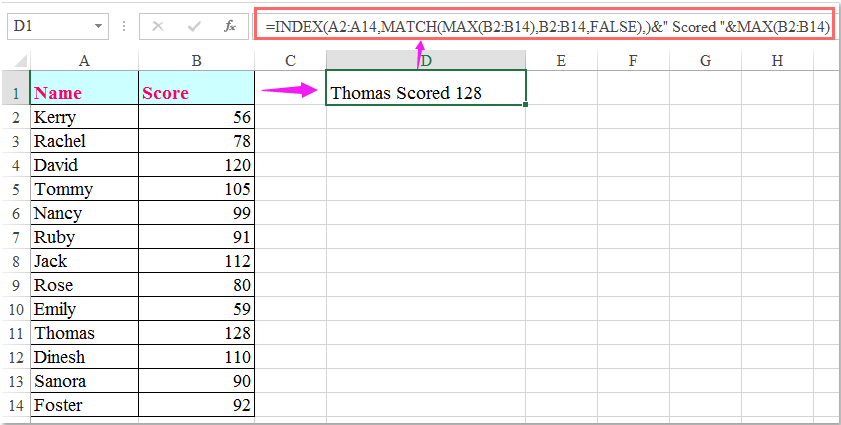
1. Enter the following formula in a blank cell where you want to display the name (for example, cell C2):
=INDEX(A2:A14,MATCH(MAX(B2:B14),B2:B14,FALSE))&" Scored "&MAX(B2:B14)After typing the formula, press Enter to confirm. The formula will return the first name it finds with the highest score. For instance, if both John and Alice scored 98, only the first occurrence will be returned with this formula.
Notes:
1. In the above formula, A2:A14 is the name list which you want to get the name from, and B2:B14 is the score list. Make sure the ranges match exactly with your data.
2. The formula returns only the first matching name. If multiple people share the highest score, you may wish to display all names; see below for a practical solution.
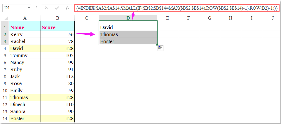
Enter the following formula into any cell (such as D2):
=INDEX($A$2:$A$14,SMALL(IF($B$2:$B$14=MAX($B$2:$B$14),ROW($B$2:$B$14)-1),ROW(B2)-1))After typing the formula, press Ctrl + Shift + Enter at the same time (not just Enter) to make it an array formula. The first name with the highest score will appear. Then, select the formula cell and drag the fill handle down. Continue dragging until error values appear – each row will display another individual who shares the highest score. This is especially useful when there are tied scores and you want to list all winners.
If your version of Excel supports dynamic arrays (such as Office365 or Excel2021 and later), you can use a more straightforward approach. Try entering this formula in a cell (and simply pressing Enter):
=FILTER(A2:A14,B2:B14=MAX(B2:B14))This formula will automatically spill all top names into the cells below, requiring no dragging or special keyboard shortcuts. It's convenient and effective for the latest Excel versions.
Formulas are powerful for quick lookups but may not be the most suitable for very large data sets, as performance can be impacted when handling thousands of rows. Additionally, formulas require consistent range references to provide correct results if rows are added or removed—so always double-check your data selection.
VBA Code - Automatically find and display name(s) for highest score
Using VBA macros offers a flexible and automated way to find and display all name(s) corresponding to the highest score in your data set, particularly when formulas become complex or insufficient for large lists. VBA allows you to customize the logic to fit report needs and handles updates automatically, making it very useful for repeated analysis or batch processing.
1. Open your Excel workbook, then click Developer > Visual Basic. In the Microsoft Visual Basic for Applications window, click Insert > Module to insert a blank module.
Copy and paste the following VBA code into the module window:
Sub ShowTopNames()
    Dim rngNames As Range, rngScores As Range, outCell As Range
    Dim nArr As Variant, sArr As Variant
    Dim i As Long, maxVal As Double, hasVal As Boolean
    Dim namesBuf As String
    On Error Resume Next
    Set rngNames = Application.InputBox("Please select the name column (single column)", "Top Names", Type:=8)
    Set rngScores = Application.InputBox("Please select the score column (single column, same rows as names)", "Top Names", Type:=8)
    Set outCell = Application.InputBox("Please select the output cell (optional, click Cancel to skip)", "Top Names", Type:=8)
    On Error GoTo 0
    If rngNames Is Nothing Or rngScores Is Nothing Then Exit Sub
    If rngNames.Rows.Count <> rngScores.Rows.Count Or rngNames.Columns.Count <> 1 Or rngScores.Columns.Count <> 1 Then
        MsgBox "Range mismatch: Name column and score column must be single columns with the same number of rows.", vbExclamation
        Exit Sub
    End If
    nArr = rngNames.Value2
    sArr = rngScores.Value2
    hasVal = False
    For i = 1 To UBound(sArr, 1)
        If IsNumeric(sArr(i, 1)) And Not IsEmpty(sArr(i, 1)) Then
            If Not hasVal Then
                maxVal = CDbl(sArr(i, 1))
                hasVal = True
            ElseIf CDbl(sArr(i, 1)) > maxVal Then
                maxVal = CDbl(sArr(i, 1))
            End If
        End If
    Next i
    If Not hasVal Then
        MsgBox "No valid numeric values found in the score column.", vbInformation
        Exit Sub
    End If
    rngNames.EntireRow.Interior.ColorIndex = xlNone
    For i = 1 To UBound(sArr, 1)
        If IsNumeric(sArr(i, 1)) Then
            If CDbl(sArr(i, 1)) = maxVal Then
                rngNames.Cells(i, 1).EntireRow.Interior.Color = RGB(255, 255, 153) ' Light yellow
                If Len(namesBuf) > 0 Then namesBuf = namesBuf & ", "
                namesBuf = namesBuf & CStr(nArr(i, 1))
            End If
        End If
    Next i
    If Not outCell Is Nothing Then
        outCell.Value = "Top Score: " & maxVal & " | Name(s): " & namesBuf
    End If
    MsgBox "Top Score = " & maxVal & vbCrLf & "Name(s): " & namesBuf, vbInformation, "Highest Score"
End Sub
2. Then, press F5 key to eun this code. You’ll see three prompts: Select the name column (single column). Drag to select just the names (e.g., A2:A14) → OK. Select the score column (single column, same rows as names). Drag to select the scores (e.g., B2:B14) → OK. Select the output cell (optional). Click a destination cell (e.g., D2) to put the result.
After the code runs, the result will be displayed in the specified cell, and the entire rows of all tied top scorers will be highlighted in light yellow.
Pivot Table - Use a pivot table to display name corresponding to the highest score
Pivot tables in Excel offer a visual and interactive way to analyze and summarize data. They are especially useful for handling larger data sets, performing group analysis, and quickly identifying unique maximum values, such as identifying the top scorer in each category or overall in a list. This method requires no formulas or coding, making it suitable for users who prefer point-and-click solutions and regular reporting tasks.
The basic workflow to use a pivot table for this requirement is as follows:
1. Select any cell within your data range (both name and score columns included), then go to Insert > PivotTable. In the dialog, confirm the data range and choose to place the pivot table on a new or existing worksheet as preferred.
2. In the PivotTable Fields pane, drag the Name field to the Rows area, and the Score field to the Values area. The Values area will by default be set to "Sum" or "Count". Click the drop-down arrow of the Score field in the Values area, select Value Field Settings, and choose Max as the summary function. Click OK.
3. Now the pivot table displays the highest score for each name. To highlight the overall top scorer, sort the "Max of Score" column in descending order—the name at the top will be the highest (or tied for highest) scorer. You can also apply filters or conditional formatting for visual emphasis.
If you want to display only the top scorer(s), apply Value Filters: click the drop-down arrow on the Row Labels for Names, select Value Filters > Equals, and set the value to the highest score (which you can identify by temporarily sorting values or checking the highest number in the Max of Score column). This allows you to focus the report on only the winning name(s).
Pivot tables are robust for exploration: you can easily update, expand, or filter your data, and the pivot table can be refreshed to automatically recalculate results. However, if your data set changes frequently, always remember to right-click your pivot table and choose Refresh after adding new data.
Pivot tables may take a little initial setup, but they offer flexible reporting and comparisons across groups, such as by department or team, should your data include extra categories.
If you experience issues with summarizing or sorting, check that your data has no blanks and that field names are spelled consistently. When large lists are in use, careful attention to the source range ensures the pivot table accounts for all relevant data.

Unlock Excel Magic with Kutools AI
- Smart Execution: Perform cell operations, analyze data, and create charts—all driven by simple commands.
- Custom Formulas: Generate tailored formulas to streamline your workflows.
- VBA Coding: Write and implement VBA code effortlessly.
- Formula Interpretation: Understand complex formulas with ease.
- Text Translation: Break language barriers within your spreadsheets.
Best Office Productivity Tools
Supercharge Your Excel Skills with Kutools for Excel, and Experience Efficiency Like Never Before. Kutools for Excel Offers Over 300 Advanced Features to Boost Productivity and Save Time. Click Here to Get The Feature You Need The Most...
Office Tab Brings Tabbed interface to Office, and Make Your Work Much Easier
- Enable tabbed editing and reading in Word, Excel, PowerPoint, Publisher, Access, Visio and Project.
- Open and create multiple documents in new tabs of the same window, rather than in new windows.
- Increases your productivity by 50%, and reduces hundreds of mouse clicks for you every day!
All Kutools add-ins. One installer
Kutools for Office suite bundles add-ins for Excel, Word, Outlook & PowerPoint plus Office Tab Pro, which is ideal for teams working across Office apps.
- All-in-one suite — Excel, Word, Outlook & PowerPoint add-ins + Office Tab Pro
- One installer, one license — set up in minutes (MSI-ready)
- Works better together — streamlined productivity across Office apps
- 30-day full-featured trial — no registration, no credit card
- Best value — save vs buying individual add-in