How to check if cell contains one of several values in Excel?

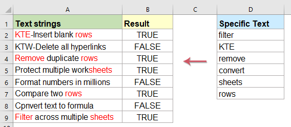
In many business, analytical, or data review scenarios, you may have a list of text strings in column A and wish to examine whether each cell contains any one of a set of specified values, such as those listed in range D2:D7. For example, in survey data, logs, or product lists, it is crucial to identify whether entries include any relevant keywords, product codes, or prohibited terms. If a cell includes any of the items from your specified list, you may want Excel to return True; otherwise, return False, as illustrated in the screenshot below. This article explains practical ways to check if a cell contains one of several values in another range, offering several approaches for different Excel versions and user needs.

Check if a cell contains one of several values from a list with formulas

Display the matches if cell contains one of several values from a list with formulas

Highlight the matches if cell contains one of several values from a list with a handy feature

Check if a cell contains one of several values using Conditional Formatting

Check if a cell contains one of several values from a list with formulas

To determine if a cell contains any of the text values from another range, you can use an array formula that works efficiently even for large datasets. This method is especially useful when you need results as logical values (True/False) for use in further formulas, filtering, or logical tests. This technique works in most modern Excel versions.

Type the following formula in a blank cell (for example, in cell B2, next to your original data), then drag the fill handle down to apply it to other cells as needed. If the cell contains any of the text values in your specified range, it returns True; otherwise, it returns False. See screenshot:

Tips and Notes:

• This formula performs a case-insensitive check. If you require case sensitivity, consider using a helper column or combining formulas in more advanced ways.
• To adapt for a “Yes” or “No” result instead of True/False, use the following adjusted formula:

• D2:D7 is your range of values (the “list”); A2 is the cell to test.
• Be mindful with blank cells or non-text data, as the SEARCH function requires a valid text input, and blank values may lead to unexpected results (“True”).

Display the matches if cell contains one of several values from a list with formulas

Sometimes, it can be more informative to display which of the values from the list actually appear in each cell, rather than simply showing a True/False result. For instance, when scanning product descriptions or comments for specific keywords, you may want to return all found values for further analysis or reporting. You can use the following formula to show all matching values separated by commas, as illustrated here:

Enter this formula into a blank cell (e.g., B2), and it will list all values from D2:D7 found within A2, separated by commas:

Note: Here, D2:D7 is the collection of values to look up, and A2 is the cell to search in.

After typing the formula, press Ctrl + Shift + Enter. Then, you can drag the fill handle down to apply the formula to other rows, as shown in the result screenshot:

• The TEXTJOIN function is available only in Excel 2019 and Office 365. In earlier versions of Excel, use the following array formula, entering it in a blank cell, and then pressing Ctrl + Shift + Enter:

Drag the formula rightward to cover as many columns as possible to capture all possible matches, and then drag down for each row. Extra columns will remain blank where there are fewer matches. This format is especially useful when you need the matches listed in separate columns:

If you encounter errors, double-check the ranges, ensure that the D2:D7 region is correct, and confirm you are using the correct delimiter for your locale (comma or semicolon).

Highlight the matches if cell contains one of several values from a list with a handy feature

If you need to visually highlight the keywords or phrases that match any value from your list within each cell, this can help make important data stand out for review or action. The Mark Keyword feature in Kutools for Excel is designed for this scenario, letting you quickly highlight any instance of your specified words in the data range without writing formulas or VBA code. In large sheets or complex datasets, this feature is especially helpful when manual inspection is impractical.

After installing Kutools for Excel, follow these steps:

1. Go to Kutools > Text > Mark Keyword to launch the dialog, as shown:

2. In the Mark Keyword dialog, carry out the following:

• Select your target data range from the Range box.
• Choose, or manually enter, the keywords in the Keyword box (separated by commas).
• Specify a highlight color using the Mark keyword colors option.

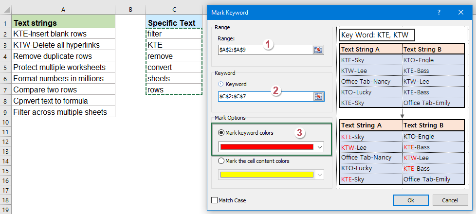
3. Click OK. All matching words within the selected range will be highlighted with your chosen font color:

• This feature directly modifies the display formatting of matched keywords, making review or sharing results more intuitive for teams who may not understand formula outputs.
• It is especially effective when the keyword list or text range is very large, or you need to highlight multiple criteria at once.
• Always double-check your selected range and keyword entries before confirming to avoid unintentional highlighting.

Check if a cell contains one of several values using Conditional Formatting

Excel's built-in Conditional Formatting is another effective approach for highlighting cells that contain any value from your specified list. This solution is useful for visually identifying relevant rows with just a glance, especially during data review, error checking, or compliance tasks. Unlike the Mark Keyword feature of Kutools, this approach does not require any add-ins, making it accessible in standard Excel installations.

Here's how to use Conditional Formatting with a formula:

• Select the cells in your data range (e.g., A2:A20) that you want to monitor.
• Go to the Home tab, click Conditional Formatting > New Rule.
• In the New Formatting Rule dialog, choose Use a formula to determine which cells to format.
• Enter this formula, assuming D2:D7 contains your values, and A2 is the first data cell:

=SUMPRODUCT(--ISNUMBER(SEARCH($D$2:$D$7,A2)))>0

• Click Format, set your desired formatting (such as fill color), and press OK.

All cells containing any item in the D2:D7 list will now be highlighted automatically.

• This method is dynamic: if you update the range D2:D7, formatting will adjust accordingly.
• Conditional formatting is view-only: it visually marks cells but does not provide results in a separate column or for further calculation.
• Formula-based conditional formatting is powerful, but with very large datasets, performance may slow down due to repeated computation.
• Be aware that SEARCH is not case-sensitive. To make this approach case-sensitive, more advanced techniques or helper columns may be needed.

More relative articles: