How to check if cell contains one of several values in Excel?

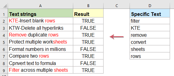
Supposing, you have a list of text strings in column A, now, you want to test each cell if it contains one of several values based on another range D2:D7. If it contains any of the specific text in D2:D7, it will display True, otherwise, it will show False as following screenshot shown. This article, I will talk about how to identify a cell if it contains one of several values in another range.

Check if a cell contains one of several values from a list with formulas

To check if a cell content contains any one of the text values in another range, the following formulas may help you, please do as this:

Enter the below formula into a blank cell where you want to locate the result, B2, for instance, then drag the fill handle down to the cells that you want to apply this formula, and if the cell has any of the text values in another specific range, it will get True, otherwise, it will get False. See screenshot:

=SUMPRODUCT(--ISNUMBER(SEARCH($D$2:$D$7,A2)))>0

Tips:

1. If you would like use “Yes” or “No’ to indicate the result, please apply the following formula, and you will get the following result as you need, see screenshot:

=IF(SUMPRODUCT(--ISNUMBER(SEARCH($D$2:$D$6,A2))),"Yes","No")

2. In the above formulas, D2:D7 is the specific data range which you want to check the cell based on, and A2 is the cell that you want to check.


Display the matches if cell contains one of several values from a list with formulas

Sotimes, you may want to check if a cell contains a value in the list and then returns that value, if multiple values match then all matching values in the list are displayed as below screenshot shown.How could you solve this task in Excel?

To display all matching vaues if the cell contains one of the specific text, please apply the below formula:

=TEXTJOIN(", ", TRUE, IF(COUNTIF(A2, "*"&$D$2:$D$7&"*"), $D$2:$D$7, ""))

Note: In the above formula, D2:D7 is the specific data range which you want to check the cell based on, and A2 is the cell that you want to check.

Then, press Ctrl + Shift + Enter keys together to get the first result, and then drag the fill handle down to the cells that you want to apply this formula, see screenshot:

Tips:

The above TEXTJOIN function only available for Excel 2019 and Office 365, if you have earlier Excel versions, you should apply the below formula:

=IFERROR(INDEX($D$2:$D$7, SMALL(IF(COUNTIF($A2, "*"&$D$2:$D$7&"*"), MATCH(ROW($D$2:$D$7), ROW($D$2:$D$7)), ""), COLUMNS($F$1:F1))), "")

Note: In the above formula, D2:D7 is the specific data range which you want to check the cell based on, and A2 is the cell that you want to check.

Then, press Ctrl + Shift + Enter keys together to get the first result, and then drag the formula cell to right side until blank cell is displayed, and then go on dragging the fill handle down to other cells, and all matching values have been displayed as below screenshot shown:


Highlight the matches if cell contains one of several values from a list with a handy feature

If you want to highlight a specific font color for the matching values if cell contains one of several values from another list, this section, I will introduce an easy feature, Mark Keyword of Kutools for Excel, with this utility, you can highlight the specific one or more keywords at once within the cells.

Note:To apply these Mark Keyword features, firstly, you should download the Kutools for Excel, and then apply the features quickly and easily.

After installing Kutools for Excel, please do as follows:

1. Click Kutools > Text > Mark Keyword, see screenshot:

2. In the Mark Keyword dialog box, please do the following operations:

  • Select the data range that you want to highlight the matching texts from the Range textbox;
  • Select the cells contains the keywords that you want to highlight based on, you can also enter the keywords manually (separate by comma) into the Keyword text box
  • At last, you should specify a font color for highlighting the texts by check Mark keyword colors option. 
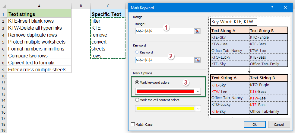
3. Then, click Ok button, all matching texts have been highlighted as below screenshot shown:


More relative articles:

  • Compare Two Or More Text Strings In Excel
  • If you want to compare two or more text strings in a worksheet with case sensitive or not case sensitive as following screenshot shown, this article, I will talk about some useful formulas for you to deal with this task in Excel.
  • If Cell Contains Text Then Display In Excel
  • If you have a list of text strings in column A, and a row of keywords, now, you need to check if the keywords are appear in the text string. If the keywords appear in the cell, displaying it, if not, blank cell is displayed as following screenshot shown.
  • Count Keywords Cell Contains Based On A List
  • If you want to count the number of keywords appears in a cell based on a list of cells, the combination of the SUMPRODUCT, ISNUMBER and SEARCH functions may help you to solve this problem in Excel.
  • Find And Replace Multiple Values In Excel
  • Normally, the Find and Replace feature can help you to find a specific text and replace it with another one, but, sometimes, you may need to find and replace multiple values simultaneously. For example, to replace all “Excel” text to “Excel 2019”, “Outlook” to “Outlook2019” and so on as below screenshot shown. This article, I will introduce a formula for solving this task in Excel.

Best Office Productivity Tools

🤖 Kutools AI Aide: Revolutionize data analysis based on: Intelligent Execution   |  Generate Code  |  Create Custom Formulas  |  Analyze Data and Generate Charts  |  Invoke Kutools Functions
Popular Features: Find, Highlight or Identify Duplicates   |  Delete Blank Rows   |  Combine Columns or Cells without Losing Data   |   Round without Formula ...
Super Lookup: Multiple Criteria VLookup    Multiple Value VLookup  |   VLookup Across Multiple Sheets   |   Fuzzy Lookup ....
Advanced Drop-down List: Quickly Create Drop Down List   |  Dependent Drop Down List   |  Multi-select Drop Down List ....
Column Manager: Add a Specific Number of Columns  |  Move Columns  |  Toggle Visibility Status of Hidden Columns  |  Compare Ranges & Columns ...
Featured Features: Grid Focus   |  Design View   |   Big Formula Bar    Workbook & Sheet Manager   |  Resource Library (Auto Text)   |  Date Picker   |  Combine Worksheets   |  Encrypt/Decrypt Cells    Send Emails by List   |  Super Filter   |   Special Filter (filter bold/italic/strikethrough...) ...
Top 15 Toolsets12 Text Tools (Add Text, Remove Characters, ...)   |   50+ Chart Types (Gantt Chart, ...)   |   40+ Practical Formulas (Calculate age based on birthday, ...)   |   19 Insertion Tools (Insert QR Code, Insert Picture from Path, ...)   |   12 Conversion Tools (Numbers to Words, Currency Conversion, ...)   |   7 Merge & Split Tools (Advanced Combine Rows, Split Cells, ...)   |   ... and more

Supercharge Your Excel Skills with Kutools for Excel, and Experience Efficiency Like Never Before. Kutools for Excel Offers Over 300 Advanced Features to Boost Productivity and Save Time.  Click Here to Get The Feature You Need The Most...

Description


Office Tab Brings Tabbed interface to Office, and Make Your Work Much Easier

  • Enable tabbed editing and reading in Word, Excel, PowerPoint, Publisher, Access, Visio and Project.
  • Open and create multiple documents in new tabs of the same window, rather than in new windows.
  • Increases your productivity by 50%, and reduces hundreds of mouse clicks for you every day!
Comments (56)
No ratings yet. Be the first to rate!
This comment was minimized by the moderator on the site
Hello,

I have spreadsheet that have some cell with following test $5655 (BIT001), $4445 (BIT002). I would like to extract every BITxxx and display in another cell with BIT001, BIT002. I'm using MID and FIND but it work only with one BIT001 and BIT002 seems to not search. How would you do it guys?
This comment was minimized by the moderator on the site
You can use text to column > Deliminate > ("("), - I will spit the text from Open Bracket .. like BIT001), then you can remove the closing bracket with a find and replace option.
This comment was minimized by the moderator on the site
Hi all,

Any suggestions...

I have a VALUE next to the SPECIFIC TEXT column F. I need a RESULT in Column B with the VALUE next to SPECIFIC TEXT.
This comment was minimized by the moderator on the site
In option "Display the matches if cell contains one of several values from a list with formulas" I'm having issues in "Result" when the "Specific Text" values is similar to others.

For example, if I have in "Specific Text" the values 'remove' and 'remove lines', I need to get in "Result" the correct value.

Thanks
This comment was minimized by the moderator on the site
I find an option in other webpage:

=TEXTJOIN(" ",1,IF(ISNUMBER(FIND(" "&$F$2:$F$6&" "," "&B2&" ")),$F$2:$F$6,""))
This comment was minimized by the moderator on the site
In the option "Display the matches if cell contains one of several values from a list with formulas" I'm having issues if the word to search is similar to other word. For example if in "Specif text" I have: Remove and Remove line, I need to get/recognise in "Result" the different values ("Remove" for 1 line and "Remove line" in other line). The problem is that always I'm getting "Remove"
This comment was minimized by the moderator on the site
Bonjour, j'essaye cette formule sur une très grande liste de mot et la recherche fait un contient, mais pas au mot entier.
Vous avez une solution ?

Par exemple, le mot de ma liste à rechercher est "aire". Cependant, le mot "horaire" m'indique vrai... avec la formule.
Alors oui "horaire" contient "aire" mais pas en mot entier...

Autre exemple : le mot de ma liste à rechercher est "ri". Cependant, le mot "clé dynamométrique" m'indique vrai...

Merci
This comment was minimized by the moderator on the site
Hello, Greg,
Sorry, I can't understand you clearly.
Could you explain your problem in English? Or you can upload a file or screenshot of your problem here.
Thank you!
This comment was minimized by the moderator on the site
=IF(SUMPRODUCT(--ISNUMBER(SEARCH($D$2:$D$6,A2))),"Yes","No")

Is there a way of amending the formula to return the number of words appear in the text examined?

e.g. returned answer is not whether one of three words (a given list) are found, but if 1, 2, or 3 words are found.

Hope this makes sense................

Thanks


Alan
This comment was minimized by the moderator on the site
Hello, Alan,
To solve your problem, the following array formula may help you: (Note: After inserting the formula, press Ctrl + Shift + Enter keys together to get the first result.)
=SUM((LEN(A2)-LEN(SUBSTITUTE(A2,$D$2:$D$5,"")))/LEN($D$2:$D$5))


Please have a try, hope it can help you!
This comment was minimized by the moderator on the site
help someone. I have a spreadsheet that has example below. I need a formula that will search and return the following based on what is in the cell

A-05-002F: Air Conditioning Unit or Heat Pump Split System - Qtrly Filter
A-11-025: Air Handler Unit - Annual
E-42-001: Emergency Generators - Weekly #4

The above is in C2 I want E2 to display Q if cell contains Qtrly, A if cell contains Annual, W if cell contains weekly
This comment was minimized by the moderator on the site
Hi, Lynda,
To solve your problem, please apply the following formula:
=IF(ISERROR(SEARCH("Qtrly",C2)),IF(ISERROR(SEARCH("Annual",C2)),IF(ISERROR(SEARCH("weekly",C2)),"","W"),"A"), "Q")

Please have a try, hope it can help you!
This comment was minimized by the moderator on the site
Correction the above information is in C2 C3 C4
This comment was minimized by the moderator on the site
RE: above example  =IFERROR(INDEX($D$2:$D$7, SMALL(IF(COUNTIF($A2, "*"&$D$2:$D$7&"*"), MATCH(ROW($D$2:$D$7), ROW($D$2:$D$7)), ""), COLUMNS($F$1:F1))), "")I keep error with Excel 2010.  Same with example for Excel 2019, in Excel 2019 on a different PC. Tried the one  Is it Wish it was available in my Kutools  
This comment was minimized by the moderator on the site
Multiple search value in a single cell, and return as a Common Value
This comment was minimized by the moderator on the site
Is it possible to do this with a partial match of the keywords? This method is only an exact match
There are no comments posted here yet
Load More
Please leave your comments in English
Posting as Guest
×
Rate this post:
0   Characters
Suggested Locations