
How to list all matched instances of a value in Excel?

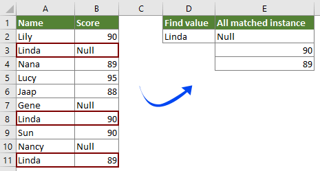
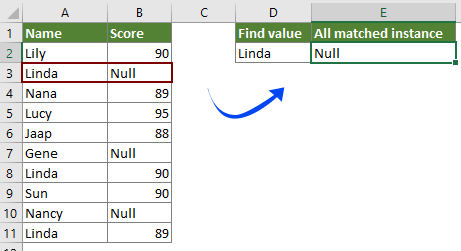
As the left screenshot shown, you need to find and list all match instances of value “Linda” in the table. How to achieve it? Please try the methods in this article.

List all matched instances of a value with array formula
Easily list only the first matched instance of a value with Kutools for Excel

More tutorials for VLOOKUP...


List all matched instances of a value with array formula

With the following array formula, you can easily list all match instances of a value in a certain table in Excel. Please do as follows.

1. Select a blank cell to output the first matched instance, enter the below formula into it, and then press the Ctrl + Shift + Enter keys simultaneously. 

=INDEX($B$2:$B$11, SMALL(IF($D$2=$A$2:$A$11, ROW($A$2:$A$11)-ROW($A$2)+1), ROW(1:1)))

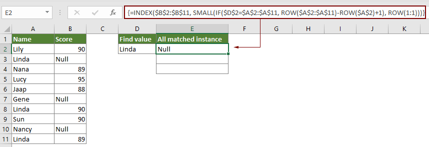
Note: In the formula, B2:B11 is the range which the matched instances locate in. A2:A11 is the range contains the certain value you will list all instances based on. And D2 contains the certain value.

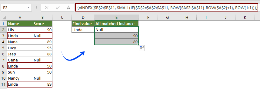
2. Keep selecting the result cell, then drag the Fill Handle down to get the other matched instances.


Easily list only the first matched instance of a value with Kutools for Excel

You can easily find and list the first matched instance of a value with the Look for a value in list function of Kutools for Excel without remembering formulas. Please do as follows.

Before applying Kutools for Excel, please download and install it firstly.

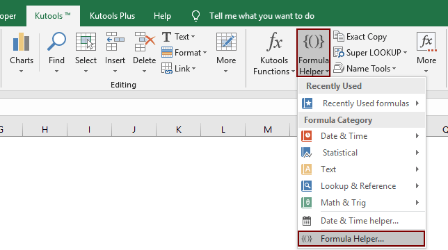
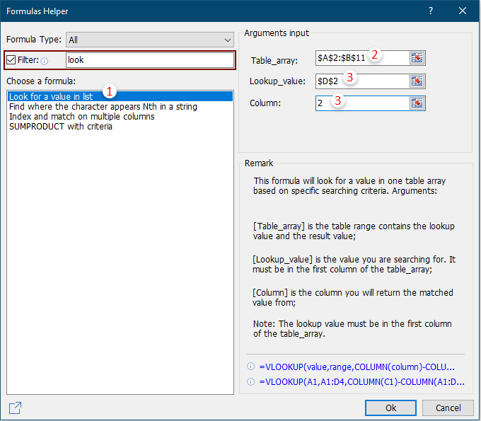
1. Select a blank cell you will place the first matched instance, then click Kutools > Formula Helper > Formula Helper

2. In the Formulas Helper dialog box, you need to:

2.1 Find and select Look for a value in list option in the Choose a formula box;
Tips: You can check the Filter box, enter the keyword into the textbox to quickly filter the formula you need.
2.2 In the Table_array box, select the table range which contains both the specific value column and matched instances column;
2.3 In the Look_value box, select the cell with the specific value you will list the first instance based on;
2.4 In the Column box, select the column contains the matched instance. Or just enter the column number into it;
Tips: The column number is based on the selected number of columns, if you select four columns, and this is the 3rd column, you need to enter number 3 into the Column box.
2.5 click the OK button. 

Then the first matched instance of the given value is listed as below screenshot shown.

  If you want to have a free trial (30-day) of this utility, please click to download it, and then go to apply the operation according above steps.


related articles

Vlookup values across multiple worksheets
You can apply the vlookup function to return the matching values in a table of a worksheet. However, if you need to vlookup value across multiple worksheets, how can you do? This article provides detailed steps to help you easily solve the problem.

Vlookup and return matched values in multiple columns
Normally, applying the Vlookup function can only return the matched value from one column. Sometimes, you may need to extract matched values from multiple columns based on the criteria. Here is the solution for you.

Vlookup to return multiple values in one cell
Normally, when applying the VLOOKUP function, if there are multiple values that match the criteria, you can only get the result of the first one. If you want to return all matched results and display them all in a single cell, how can you achieve?

Vlookup and return entire row of a matched value
Normally, using the vlookup function can only return a result from a certain column in the same row. This article is going to show you how to return the whole row of data based on specific criteria.

Backwards Vlookup or in reverse order
In general, the VLOOKUP function searches values from left to right in the array table, and it requires the lookup value must stay in the left side of target value. But, sometimes you may know the target value and want to find out the lookup value in reverse. Therefore, you need to vlookup backwards in Excel. There are several ways in this article to deal with this problem easily!

More tutorials for VLOOKUP...

Best Office Productivity Tools

🤖 Kutools AI Aide: Revolutionize data analysis based on: Intelligent Execution   |  Generate Code  |  Create Custom Formulas  |  Analyze Data and Generate Charts  |  Invoke Kutools Functions
Popular Features: Find, Highlight or Identify Duplicates   |  Delete Blank Rows   |  Combine Columns or Cells without Losing Data   |   Round without Formula ...
Super Lookup: Multiple Criteria VLookup    Multiple Value VLookup  |   VLookup Across Multiple Sheets   |   Fuzzy Lookup ....
Advanced Drop-down List: Quickly Create Drop Down List   |  Dependent Drop Down List   |  Multi-select Drop Down List ....
Column Manager: Add a Specific Number of Columns  |  Move Columns  |  Toggle Visibility Status of Hidden Columns  |  Compare Ranges & Columns ...
Featured Features: Grid Focus   |  Design View   |   Big Formula Bar    Workbook & Sheet Manager   |  Resource Library (Auto Text)   |  Date Picker   |  Combine Worksheets   |  Encrypt/Decrypt Cells    Send Emails by List   |  Super Filter   |   Special Filter (filter bold/italic/strikethrough...) ...
Top 15 Toolsets12 Text Tools (Add Text, Remove Characters, ...)   |   50+ Chart Types (Gantt Chart, ...)   |   40+ Practical Formulas (Calculate age based on birthday, ...)   |   19 Insertion Tools (Insert QR Code, Insert Picture from Path, ...)   |   12 Conversion Tools (Numbers to Words, Currency Conversion, ...)   |   7 Merge & Split Tools (Advanced Combine Rows, Split Cells, ...)   |   ... and more

Supercharge Your Excel Skills with Kutools for Excel, and Experience Efficiency Like Never Before. Kutools for Excel Offers Over 300 Advanced Features to Boost Productivity and Save Time.  Click Here to Get The Feature You Need The Most...

Description


Office Tab Brings Tabbed interface to Office, and Make Your Work Much Easier

  • Enable tabbed editing and reading in Word, Excel, PowerPoint, Publisher, Access, Visio and Project.
  • Open and create multiple documents in new tabs of the same window, rather than in new windows.
  • Increases your productivity by 50%, and reduces hundreds of mouse clicks for you every day!
Comments (15)
Rated 5 out of 5 · 1 ratings
This comment was minimized by the moderator on the site
Is there a way to make it totla up the values it find and just put it in the first box?
This comment was minimized by the moderator on the site
Hi Bramdon,

To total up all matched values, the following formula can help. Or you can take a look at this tutorial: vlookup and sum matches in rows or columns in Excel
=SUMPRODUCT((A2:A7=A10)*B2:F7)
https://www.extendoffice.com/images/stories/doc-excel/doc-vlookup-and-sum/doc-vlookup-sum-sumif4.png
This comment was minimized by the moderator on the site
Is there a way to stop this formula returning duplicate values

Thanks
Steven
This comment was minimized by the moderator on the site
Hi Steven Waddleton,
The following two formulas can do you a favor.
Array formula in E2:
=INDEX($B$2:$B$11,MATCH(0,COUNTIF($E$1:E1,$B$2:$B$11)+($A$2:$A$11<>$D$2),0)) + Ctrl + Shift + Enter
Formula in E2:
=LOOKUP(2, 1/((COUNTIF($F$1:F1,$B$2:$B$11)=0)*($D$2=$A$2:$A$11)), $B$2:$B$11)
In the formulas, E1 is the cell above the result cell.
https://www.extendoffice.com/images/stories/comments/comment-picture-zxm/instance-no-duplicates.png
This comment was minimized by the moderator on the site
WOW! Worked perfectly, thanks a ton! Awesome formula.
Rated 5 out of 5
This comment was minimized by the moderator on the site
Nice formula. In testing it I get #NUMBER! when I clear cells A9:B11. How to change the formula to prevent getting this error? I wonder, because I want to use this formula for a list of events on a certain date and on date 1 there are 40 events, on day 2 it are 10 events etc. I could create an indexed list for perhaps 100 rows, but it looks very strange when for date 2 the first 10 rows show events and the other 90 rows show #NUMBER!. It would be okay for me if it gave "-" as a result instead of #NUMBER!
This comment was minimized by the moderator on the site
Fantastic. Thank you so much. Very helpful for my work.
This comment was minimized by the moderator on the site
Amazing. The formula worked for me exactly the way I was looking for. Hats off. Thanks a ton
This comment was minimized by the moderator on the site
Question, I have a sheet laid out opposite of this where "Linda" would be the column header I would like to flag on and the value "90" or 89" I would like to return. Would I change the row function to a column function?
This comment was minimized by the moderator on the site
How would I use this formula but instead of filling down I could fill across but the formula would continue moving down as I fill across (ie. the formula changes from ROW(1:1) to ROW(2:2)
This comment was minimized by the moderator on the site
Hi Luke,The below array formula can do you a favor. Note: After entering the formula, please press the Ctrl + Shift + Enter key to apply it. And then drag its Fill Handle right across the cells you need. =INDEX($B$2:$B$11, SMALL(IF($D$2=$A$2:$A$11, ROW($A$2:$A$11)-ROW($A$2)+1), COLUMN(A1)))
This comment was minimized by the moderator on the site
A very useful and educational formula. I am matching against a set numeric value and it works a treat. How can I use >= rather than just = (i.e. IF($D$2>=$A$2:$A$11) to perform the match so it is looking for values greater than a set value (in $D$2). I assume as it doesn't work as one of the functions in the formula is matching against specific text rather than working with numbers?
This comment was minimized by the moderator on the site
This was super useful, thanks! I'm trying to take this one step further and be able to return all match instances of a certain value while having to search through more than a single-column array. To work through this using your example, I added a second column of test scores and modified your formula to look up a given test score and return the names that match that score. I got this to work with INDEX(SMALL()) and can pull all of the names from both test columns. I've also managed to return only names with that score on Test 2 using INDEX(MATCH(INDEX(MATCH))), however this can only find the first instance in the array. What I'm really trying to do is a combination of these: return all of the names with the given array, while narrowing the search to a specific column within the array. Do you have any tips for this?
This comment was minimized by the moderator on the site
Good day,
Would you please provide a screenshot of your spreadsheet showing what you are exactly trying to do? Thank you for your comment.
There are no comments posted here yet
Load More
Please leave your comments in English
Posting as Guest
×
Rate this post:
0   Characters
Suggested Locations