How to highlight cell or row with checkbox in Excel?
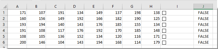
As shown in the screenshot below, you need to highlight a row or cell with a checkbox. When a checkbox is checked, a specified row or a cell will be highlighted automatically. But how to achieve it in Excel? This article will show you two methods to achieve it.

Highlight cell or row with checkbox with Conditional Formatting
Highlight cell or row with checkbox with VBA code
Highlight cell or row with checkbox with Conditional Formatting
You can create a Conditional Formatting rule to highlight cell or row with checkbox in Excel. Please do as follows.
Step ONE: Link all check box to a specified cell
1. You need to insert checkboxes into cells one by one manually by clicking Developer > Insert > Check Box(Form Control).
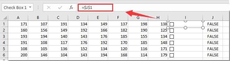
2. Now check boxes have been inserted to cells in column I. Please select the first check box in I1, enter formula =$J1 into the formula bar, and then press the Enter key.
Tip: If you don't want to have values associated in adjacent cells to checkboxes, you can link the checkbox to another worksheet's cell such as =Sheet3!$E1.
3. Repeat step 1 until all check boxes are linked to the adjacent cells or cells in another worksheet.
Note: All linked cells should be consecutive and locating in the same column.
Step TWO: Create a Conditional Formatting rule
Now you need to create a Conditional Formatting rule as follows step by step.
1. Select the rows you need to highlight with checkboxes, then click Conditional Formatting > New Rule under the Home tab. See screenshot:

2. In the New Formatting Rule dialog box, you need to:
2.1 Select the Use a formula to determine which cells to format option in the Select a Rule Type box;
2.2 Enter formula =IF($J1=TRUE,TRUE,FALSE) into the Format values where this formula is true box;
Or =IF(Sheet3!$E1=TRUE,TRUE,FALSE) if the check boxes linked to another worksheet.
2.3 Click the Format button to specify a highlighted color for the rows;
2.4 Click the OK button. See screenshot:

Note: In the formula, $J1 or $E1 is the first linked cell for the check boxes, and make sure the cell reference has been changed to column absolute (J1 > $J1 or E1 > $E1).
Now the Conditional Formatting rule is created. When checking the check boxes, the corresponding rows will be highlighted automatically as bellows screenshot shown.

Highlight cell or row with checkbox with VBA code
The following VBA code can also help you to highlight cell or row with checkbox in Excel. Please do as follows.
1. In the worksheet you need to highlight cell or row with checkbox. Right click the Sheet Tab and select View Code from the right-clicking menu to open the Microsoft Visual Basic for Applications window.
2. Then copy and paste the below VBA code into the Code window.
VBA code: Highlight row with checkbox in Excel
Sub AddCheckBox()
Dim xCell As Range
Dim xRng As Range
Dim I As Integer
Dim xChk As CheckBox
On Error Resume Next
InputC:
    Set xRng = Application.InputBox("Please select the column range to insert checkboxes:", "Kutools for Excel", Selection.Address, , , , , 8)
If xRng Is Nothing Then Exit Sub
If xRng.Columns.Count > 1 Then
    MsgBox "The selected range should be a single column", vbInformation, "Kutools fro Excel"
    GoTo InputC
Else
    If xRng.Columns.Count = 1 Then
        For Each xCell In xRng
            With ActiveSheet.CheckBoxes.Add(xCell.Left, _
               xCell.Top, xCell.Width = 15, xCell.Height = 12)
               .LinkedCell = xCell.Offset(, 1).Address(External:=False)
               .Interior.ColorIndex = xlNone
               .Caption = ""
               .Name = "Check Box " & xCell.Row
            End With
            xRng.Rows(xCell.Row).Interior.ColorIndex = xlNone
        Next
    End If
    With xRng
     .Rows.RowHeight = 16
    End With
    xRng.ColumnWidth = 5#
    xRng.Cells(1, 1).Offset(0, 1).Select
    For Each xChk In ActiveSheet.CheckBoxes
      xChk.OnAction = ActiveSheet.Name + ".InsertBgColor"
    Next
End If
End Sub

Sub InsertBgColor()
Dim xName As Integer
Dim xChk As CheckBox
For Each xChk In ActiveSheet.CheckBoxes
  xName = Right(xChk.Name, Len(xChk.Name) - 10)
  If (xName = Range(xChk.LinkedCell).Row) Then
   If (Range(xChk.LinkedCell) = "True") Then
    Range("A" & xName, Range(xChk.LinkedCell).Offset(0, -2)).Interior.ColorIndex = 6
   Else
    Range("A" & xName, Range(xChk.LinkedCell).Offset(0, -2)).Interior.ColorIndex = xlNone
   End If
  End If
Next
End Sub
3. Press the F5 key to run the code. (Note: you should put the cursor into the first part of the code to apply the F5 key) In the popping up Kutools for Excel dialog box, please select the range you want to insert check boxes, and then click the OK button. Here I select range I1:I6. See screenshot:

4. Then check boxes are inserted into selected cells. Check any one of the checkboxes, the corresponding row will be highlighted automatically as below screenshot shown.

Related articles:
- How to change a specified cell value or color when checkbox is checked in Excel?
- How to insert date stamp into a cell if ticked a checkbox in Excel?
- How to make checkbox checked based on cell value in Excel?
- How to filter data based on checkbox in Excel?
- How to hide checkbox when row is hidden in Excel?
- How to create a drop down list with multiple checkboxes in Excel?
Best Office Productivity Tools
Supercharge Your Excel Skills with Kutools for Excel, and Experience Efficiency Like Never Before. Kutools for Excel Offers Over 300 Advanced Features to Boost Productivity and Save Time. Click Here to Get The Feature You Need The Most...
Office Tab Brings Tabbed interface to Office, and Make Your Work Much Easier
- Enable tabbed editing and reading in Word, Excel, PowerPoint, Publisher, Access, Visio and Project.
- Open and create multiple documents in new tabs of the same window, rather than in new windows.
- Increases your productivity by 50%, and reduces hundreds of mouse clicks for you every day!
All Kutools add-ins. One installer
Kutools for Office suite bundles add-ins for Excel, Word, Outlook & PowerPoint plus Office Tab Pro, which is ideal for teams working across Office apps.
- All-in-one suite — Excel, Word, Outlook & PowerPoint add-ins + Office Tab Pro
- One installer, one license — set up in minutes (MSI-ready)
- Works better together — streamlined productivity across Office apps
- 30-day full-featured trial — no registration, no credit card
- Best value — save vs buying individual add-in