How to calculate quarter and year from date in Excel?
If you have a column of date, now, you want to convert the date to quarter and year only to get the following result. Are there any quick ways to solve it in Excel?
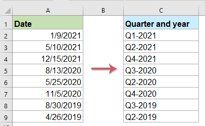
Convert date to quarter and year with formula
Here is a simple formula can help you to calculate the quarter and year from the given date, please do as follows:
Enter the following formula into a blank cell where you want to output the calculate result, and then drag the fill handle down to the cells to apply this formula, and the date has been displayed in quarter and year format, see screenshot:

Convert date to quarter only with formula
If you just want to get the quarter from the given date, please apply the below formula:
Then, drag the fill handle down to the cells for filling this formula, only the quarter is displayed based on the date, see screenshot:

Convert date to quarter and year with a handy feature
If you have Kutools for Excel, with its Convert date to quarter feature, you can get the quarter and year format from te specific dates without remembering any formulas.
After installing Kutools for Excel, please do as follows:
1. Click to select a cell where you want to output the result, see screenshot:

2. And then click Kutools > Formula Helper > Formula Helper, see screenshot:

3. In the Formulas Helper dialog box, please do the following operations:
- Select Date from the Formula Type drop down list;
- In the Choose a formula list box, click to select Convert date to quarter option;
- Then, in the Arguments input section, select the cell containing the date that you want to convert in the Date textbox.

4. And then, click Ok button, the first result will be calculated, then drag the fill handle for fill the formula to other cells, see screenshot:

Convert quarter and year to date with formula
Sometimes, you may want to convert the quarter and year format cells to the normal date which is the first day of quarter as below screenshot shown:

For getting the first day of quarter from the quarter and year cell, please apply the below formula:
Then, drag the fill handle down to the cells for filling this formula, and all the fist days of quarter have been extracted at once, see screenshot:

More relative articles:
- Extract Month And Year Only From Date In Excel
- If you have a list of date format, now, you want to extract only the month and year from date as left screenshot shown, how could you extract month and year from the date quickly and easily in Excel?
- Sum Values Based On Month And Year In Excel
- If you have a range of data, column A contains some dates and column B has the number of orders, now, you need to sum the numbers based on month and year from another column. In this case, I want to calculate the total orders of January 2016 to get the following result. And this article, I will talk about some tricks to solve this job in Excel.
- Calculate The Difference Between Two Dates In Days, Weeks, Months And Years
- When dealing with the dates in a worksheet, you may need to calculate the difference between two given dates for getting the number of days, weeks, months or years. This article, I will talk about how to solve this task in Excel.
- Calculate Number Of Days In A Month Or A Year In Excel
- As we all know, there are leap years and common years where leap year has 366 days and common year has 365 days. To calculate the number of days in a month or a year based on a date as below screenshot shown, this article will help you.
Best Office Productivity Tools
Supercharge Your Excel Skills with Kutools for Excel, and Experience Efficiency Like Never Before. Kutools for Excel Offers Over 300 Advanced Features to Boost Productivity and Save Time. Click Here to Get The Feature You Need The Most...
Office Tab Brings Tabbed interface to Office, and Make Your Work Much Easier
- Enable tabbed editing and reading in Word, Excel, PowerPoint, Publisher, Access, Visio and Project.
- Open and create multiple documents in new tabs of the same window, rather than in new windows.
- Increases your productivity by 50%, and reduces hundreds of mouse clicks for you every day!
All Kutools add-ins. One installer
Kutools for Office suite bundles add-ins for Excel, Word, Outlook & PowerPoint plus Office Tab Pro, which is ideal for teams working across Office apps.
- All-in-one suite — Excel, Word, Outlook & PowerPoint add-ins + Office Tab Pro
- One installer, one license — set up in minutes (MSI-ready)
- Works better together — streamlined productivity across Office apps
- 30-day full-featured trial — no registration, no credit card
- Best value — save vs buying individual add-in