How to insert image or picture dynamically in cell based on cell value in Excel?

In many cases, you may need to insert image dynamically in cell based on cell value. For example, you want the corresponding images to be dynamically changed with the different values you entering in a specified cell. This article will show you how to achieve it.

Insert and change image dynamically based on the values you entering in a cell
Dynamically change image Based On Cell Values With an amazing tool

Insert and change image dynamically based on the values you entering in a cell

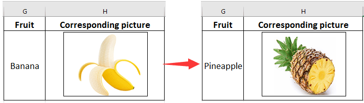
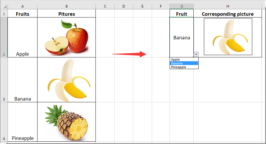
As below screenshot shown, you want to display corresponding pictures dynamically based on the value you entered in cell G2. When entering Banana in cell G2, the banana picture will be displayed in cell H2. While entering Pineapple in cell G2, the picture in cell H2 will turn into the corresponding pineapple picture.

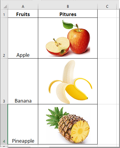
1. Create two columns in your worksheet, the first column range A2:A4 contains the name of the pictures, and the second column range B2:B4 contains the corresponding pictures. See screenshot shown.

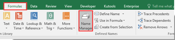
2. Click Formulas > Name Manager.

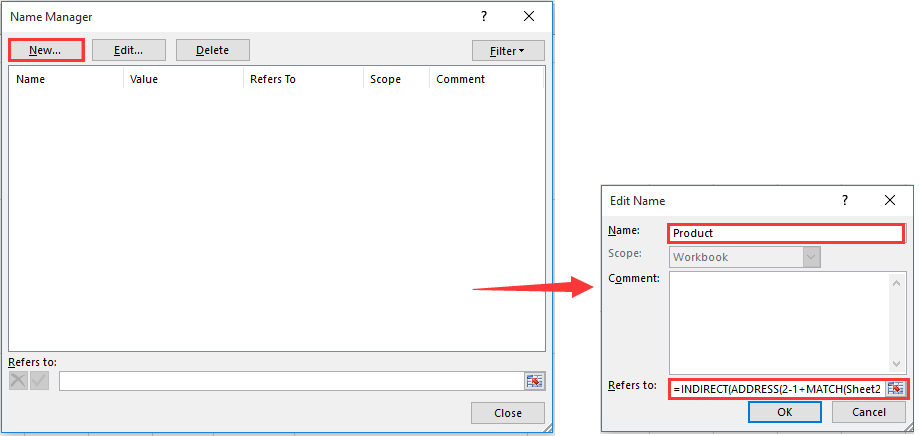
3. In the Name Manager dialog box, click the New button. Then the Edit Name dialog pops up, enter Product into the Name box, enter the below formula into the Refers to box, and then click the OK button. See screenshot:

=INDIRECT(ADDRESS(2-1+MATCH(Sheet2!$G$2, Sheet2!$A$2:$A$4, 0), 2))

Notes:

You can change them as you need in the above formula.

4. Close the Name Manager dialog box.

5. Select a picture in your Pictures column, and press Ctrl + C keys simultaneously to copy it. Then paste it to a new place in current worksheet. Here I copy the apple picture and place it in cell H2.

6. Enter a fruit name such as Apple in cell G2, click to select the pasted picture, and enter formula =Product into the Formula Bar, then press the Enter key. See screenshot:

From now on, when changing to any fruit name in cell G2, pictures in cell H2 will turn into corresponding one dynamically.

You can pick the fruit name quickly by creating a drop-down list containing all fruit names in cell G2 as below screenshot shown.

Easily insert images to related cells based on cell values with an amazing tool

For many Excel newbies, the above method is not easy to handle. Here recommend the Picture Drop-down List feature of Kutools for Excel. With this feature, you can easily create a dynamic drop-down list with values and pictures totally matching.

Please do as follows to apply the Picture Drop-down List feature of Kutools for Excel to create a dynamic picture drop-down list in Excel.

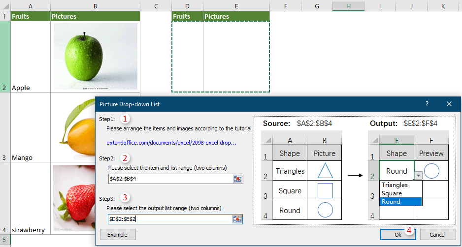
1. Firstly, you need to create two columns separately containing the values and its corresponding pictures as the below screenshot shown.

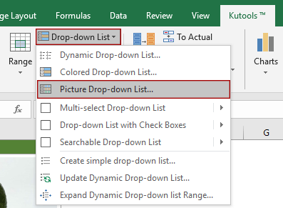
2. Click Kutools > Import & Export > Match Import Pictures.

3. In the Picture Drop-down List dialog box, you need to configure as follows.

4. Then a Kutools for Excel dialog box pops up to reminds you that some intermediate data will be created during the process, click Yes to continue.

Then a dynamic picture drop-down list is created. The picture will change dynamically based on the item you selected in the drop-down list.

Click to know more about this feature...

Related articles:

• How to create dynamic hyperlink to another sheet in Excel?
• How to dynamically extract a list of unique values from a column range in Excel?
• How to create a dynamic monthly calendar in Excel?