How to highlight the closest value in a list to a given number in Excel?
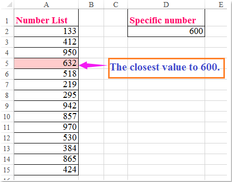
Supposing, you have a list of numbers, now, you may want to highlight the closest or several closest values based on a given number as following screenshot shown. Here, this article may help you to solve this task with ease.
Highlight the closest or closest n values to a given number with Conditional Formatting
 Highlight the closest or closest n values to a given number with Conditional Formatting
To highlight the closest value based on the given number, please do as follows:
1. Select the number list that you want to highlight, and then click Home > Conditional Formatting > New Rule, see screenshot:

2. In the New Formatting Rule dialog box, do the following operations:
(1.) Click Use a formula to determine which cells to format under the Select a Rule Type list box;
(2.) In the Format values where this formula is true text box, please enter this formula: =ABS(A2-$D$2)=MIN(ABS($A$2:$A$15-$D$2)) (A2 is the first cell in your data list, D2 is the given number you will compare, A2:A15 is the number list you want to highlight the closest value from.)

3. Then click Format button to go the Format Cells dialog box, under the Fill tab, choose one color you like, see screenshot:

4. And then click OK > OK to close the dialogs, the closest value to the specific number has been highlighted at once, see screenshot:

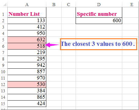
Tips: If you want to highlight the closest 3 values to the given values, you can apply this formula in the Conditional Formatting, =ISNUMBER(MATCH(ABS($D$2-A2),SMALL(ABS($D$2-$A$2:$A$15),ROW($1:$3)),0)), see screenshot:

Note: In the above formula: A2 is the first cell in your data list, D2 is the given number you will compare, A2:A15 is the number list you want to highlight the closest value from, $1:$3 indicates that the closest three values will be highlighted. You can change them to your need.

Unlock Excel Magic with Kutools AI
- Smart Execution: Perform cell operations, analyze data, and create charts—all driven by simple commands.
- Custom Formulas: Generate tailored formulas to streamline your workflows.
- VBA Coding: Write and implement VBA code effortlessly.
- Formula Interpretation: Understand complex formulas with ease.
- Text Translation: Break language barriers within your spreadsheets.
Best Office Productivity Tools
Supercharge Your Excel Skills with Kutools for Excel, and Experience Efficiency Like Never Before. Kutools for Excel Offers Over 300 Advanced Features to Boost Productivity and Save Time. Click Here to Get The Feature You Need The Most...
Office Tab Brings Tabbed interface to Office, and Make Your Work Much Easier
- Enable tabbed editing and reading in Word, Excel, PowerPoint, Publisher, Access, Visio and Project.
- Open and create multiple documents in new tabs of the same window, rather than in new windows.
- Increases your productivity by 50%, and reduces hundreds of mouse clicks for you every day!
All Kutools add-ins. One installer
Kutools for Office suite bundles add-ins for Excel, Word, Outlook & PowerPoint plus Office Tab Pro, which is ideal for teams working across Office apps.
- All-in-one suite — Excel, Word, Outlook & PowerPoint add-ins + Office Tab Pro
- One installer, one license — set up in minutes (MSI-ready)
- Works better together — streamlined productivity across Office apps
- 30-day full-featured trial — no registration, no credit card
- Best value — save vs buying individual add-in