How to sum based on column and row criteria in Excel?
I have a range of data which contains row and column headers, now, I want to take a sum of the cells that meet both column and row header criteria. For example, to sum the cells which column criteria is Tom and the row criteria is Feb as following screenshot shown. This article, I will talk about some useful formulas to solve it.
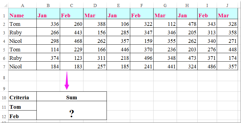
Sum cells based on column and row criteria with formulas
 Sum cells based on column and row criteria with formulas
Here, you can apply the following formulas to sum the cells based on both the column and row criteria, please do as this:
Enter any one of the below formulas into a blank cell where you want to output the result:
=SUMPRODUCT((A2:A7="Tom")*(B1:J1="Feb")*(B2:J7))
=SUM(IF(B1:J1="Feb",IF(A2:A7="Tom",B2:J7)))
And then press Shift + Ctrl + Enter keys together to get the result, see screenshot:
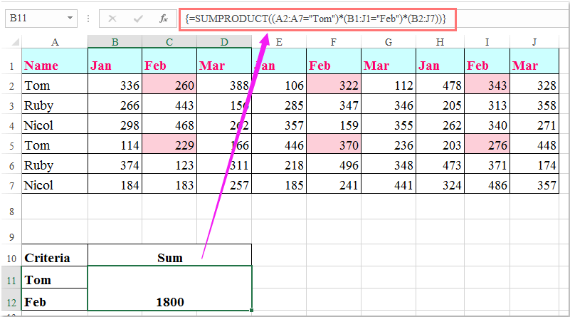
Note: In the above formulas: Tom and Feb are the column and row criteria that based on, A2:A7, B1:J1are the column headers and row headers contain the criteria, B2:J7 is the data range that you want to sum.

Unlock Excel Magic with Kutools AI
- Smart Execution: Perform cell operations, analyze data, and create charts—all driven by simple commands.
- Custom Formulas: Generate tailored formulas to streamline your workflows.
- VBA Coding: Write and implement VBA code effortlessly.
- Formula Interpretation: Understand complex formulas with ease.
- Text Translation: Break language barriers within your spreadsheets.
Best Office Productivity Tools
Supercharge Your Excel Skills with Kutools for Excel, and Experience Efficiency Like Never Before. Kutools for Excel Offers Over 300 Advanced Features to Boost Productivity and Save Time. Click Here to Get The Feature You Need The Most...
Office Tab Brings Tabbed interface to Office, and Make Your Work Much Easier
- Enable tabbed editing and reading in Word, Excel, PowerPoint, Publisher, Access, Visio and Project.
- Open and create multiple documents in new tabs of the same window, rather than in new windows.
- Increases your productivity by 50%, and reduces hundreds of mouse clicks for you every day!
All Kutools add-ins. One installer
Kutools for Office suite bundles add-ins for Excel, Word, Outlook & PowerPoint plus Office Tab Pro, which is ideal for teams working across Office apps.
- All-in-one suite — Excel, Word, Outlook & PowerPoint add-ins + Office Tab Pro
- One installer, one license — set up in minutes (MSI-ready)
- Works better together — streamlined productivity across Office apps
- 30-day full-featured trial — no registration, no credit card
- Best value — save vs buying individual add-in