How to look up a value and return the cell above or below in Excel?

In Excel, we use VLOOKUP function to find a specific value from a range data, but do you know how to look up a value and then return its above or below values? Actually, you can use INDEX function to handle it.

Look up a value and return the cell above or below


arrow blue right bubble Look up a value and return the cell above or below

Look up a value and return cell above

Select a blank cell that you want to place the return value, and type this formula =INDEX(A1:A8,MATCH(D1,A1:A8,0)-1,1), press Enter key to return the value. See screenshot:
doc look return cell above 1

Look up a value and return cell below

Select a blank cell that you want to place the return value, and type this formula =INDEX(A1:A8,MATCH(D1,A1:A8,0)+1,1), press Enter key to get the result. See screenshot:
doc look return cell above 2

Note: in the formulas, the first A1:A8 is the range where you look up for value, and the second A1:A8 is the range where you want to look up for the criterion, D1 is the value you look up, 1 indicate the column number you want to return.

If you want to look up for a value and return below and the 3 cells to the right of the reference, you can apply this formula =INDEX(F1:H8,MATCH(K1,F1:F8,0)+1,3).
doc look return cell above 3

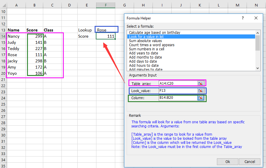
Tip.If you want to quickly lookup a value and return in another column, please try to use the Kutools for Excel’s Look for a value in list as shown in the following screenshot. It’s full function without limitation in 60 days, please download and have a free trial now.
doc look return cell above 4

Best Office Productivity Tools

🤖 Kutools AI Aide: Revolutionize data analysis based on: Intelligent Execution   |  Generate Code  |  Create Custom Formulas  |  Analyze Data and Generate Charts  |  Invoke Kutools Functions
Popular Features: Find, Highlight or Identify Duplicates   |  Delete Blank Rows   |  Combine Columns or Cells without Losing Data   |   Round without Formula ...
Super Lookup: Multiple Criteria VLookup    Multiple Value VLookup  |   VLookup Across Multiple Sheets   |   Fuzzy Lookup ....
Advanced Drop-down List: Quickly Create Drop Down List   |  Dependent Drop Down List   |  Multi-select Drop Down List ....
Column Manager: Add a Specific Number of Columns  |  Move Columns  |  Toggle Visibility Status of Hidden Columns  |  Compare Ranges & Columns ...
Featured Features: Grid Focus   |  Design View   |   Big Formula Bar    Workbook & Sheet Manager   |  Resource Library (Auto Text)   |  Date Picker   |  Combine Worksheets   |  Encrypt/Decrypt Cells    Send Emails by List   |  Super Filter   |   Special Filter (filter bold/italic/strikethrough...) ...
Top 15 Toolsets12 Text Tools (Add Text, Remove Characters, ...)   |   50+ Chart Types (Gantt Chart, ...)   |   40+ Practical Formulas (Calculate age based on birthday, ...)   |   19 Insertion Tools (Insert QR Code, Insert Picture from Path, ...)   |   12 Conversion Tools (Numbers to Words, Currency Conversion, ...)   |   7 Merge & Split Tools (Advanced Combine Rows, Split Cells, ...)   |   ... and more

Supercharge Your Excel Skills with Kutools for Excel, and Experience Efficiency Like Never Before. Kutools for Excel Offers Over 300 Advanced Features to Boost Productivity and Save Time.  Click Here to Get The Feature You Need The Most...

Description


Office Tab Brings Tabbed interface to Office, and Make Your Work Much Easier

  • Enable tabbed editing and reading in Word, Excel, PowerPoint, Publisher, Access, Visio and Project.
  • Open and create multiple documents in new tabs of the same window, rather than in new windows.
  • Increases your productivity by 50%, and reduces hundreds of mouse clicks for you every day!
Comments (34)
No ratings yet. Be the first to rate!
This comment was minimized by the moderator on the site
Hi, I need help with this excel formula. I want to the display largest values with their corresponding names, i have 3 names with the same name value but my formula returns only 1 name for all the 3 values. =INDEX(Client,MATCH(L6,Month,0)).
This comment was minimized by the moderator on the site
Hi there... what formula can I use to say .. if the sum of a formula in a cell is greater than a number then return the amount greater than 48 in the cell below?
This comment was minimized by the moderator on the site
Hi, Cindy, I do not know how your data display. Here I have a formula =INDEX(G1:G6,MATCH(IF(I1>100,MIN(IF(G1:G6>K1,G1:G6))),G1:G6,0)+1,1) which use for this example:
In G1:G6, it lists some products and prices, in I1 is the sum of a formula, in K1 type 48 into it. Then suppose that if the sum is greater than 100, it will show the cell contents below the value that greater than 48 of list G1:G6. See screenshot:
https://www.extendoffice.com/images/stories/comments/sun-comment/doc-formula-2.png
If you just want to return the number which is greater than 48 when the sum is greater than 100, use formula =IF(I1>100,MIN(IF(G1:G6>K1,G1:G6)))
This comment was minimized by the moderator on the site
Hi,
Using MS-Excel I want a separate list of numbers from each column which are coming after 22.


22 54 49 94
34 88 18 22
92 48 22 86
22 63 83 31
89 15 76 5
71 89 33 84
86 77 79 22
1 22 88 12
71 68 22 75
7 74 36 59
74 39 98 63
52 66 22 58
22 31 26 0
67 16 60 13
14 33 16 77
37 37 25 1

Pls help.
Thankyou.
This comment was minimized by the moderator on the site
Hi, I do not understand your question. May you describe your quetion with more details, or give me a before and after comparison.
This comment was minimized by the moderator on the site
Hi, I am wanting to pick a state then pick how many kgs and then it references the Price per weight listed as it changes from point to point
0-500 501-1000 1001-5000 50001-1000 10001-2200 22000+
TBRI 0.476 0.282 0.219 0.197 0.177 0.159
TCNS 0.26 0.154 0.114 0.106 0.099 0.085
TGLD 0.246 0.146 0.108 0.097 0.087 0.059
TGOL 0.605 0.485 0.387 0.287 0.213 0.197
TMCK 0.1 0.077 0.006 0.048 0.04 0.029
PPP 0.246 0.146 0.108 0.097 0.087 0.059
TRTN 0.187 0.111 0.082 0.074 0.066 0.055
TTSV 0.187 0.111 0.082 0.074 0.066 0.245
TSYD 0.562 0.376 0.342 0.308 0.277 0.259
TNTL 0.427 0.286 0.26 0.299 0.278 0.259
TWLG 0.834 0.523 0.444 0.399 0.359 0.31
This comment was minimized by the moderator on the site
Hi, i´m having the following issue, i m using the MIN function to retrieve the smallest value of a row but i m not able to retrieve the value of the cell next to the smallest

0,82 € 690 0,92 € 721 0,61 € 2446 0,71 € 2443 114 2212

each of these values are in a cell and what i need is for ex: smallest value is 0.61 so i want to retrieve the cell right next to it 2443. im using Office 2010. thanks a lot
This comment was minimized by the moderator on the site
Hi, Paulo, if all your data is in a row, and each of them in a single cell, you can try this formula: =INDIRECT(CELL("address",INDEX(A1:J1,MATCH(MIN(A1:J1),A1:J1,0)+1))), if your data is in to columns, such as:
0,82 690
0,92 721
0,61,2446
0,71 2443
114 2212
you can visit this tutorial How To VLOOKUP The Lowest Value And Return Adjacent Cell In Excel?, it will hel you.
This comment was minimized by the moderator on the site
I can only get this formula to perform by putting the MATCH clause in additional parentheses so as to carry out the arithmetic function. Otherwise it returns a #VALUE error.

Original: =INDEX(A1:A8,MATCH(D1,A1:A8,0)-1,1)
Corrected: =INDEX(A1:A8,(MATCH(D1,A1:A8,0))-1,1)
This comment was minimized by the moderator on the site
I'm trying to figure out a way to bring a customer number (text field) by looking up the invoice number. See below. I want to go to another sheet and if cell equals 6491 then return customer number 007517 (text field), and if cell equals 6487 return 009897

6491 007517
6491 007517
6486 007517
6481 009897
6487 009897
6481 009897
6480 009897

Any help would be appreciated.

Thank you!!
This comment was minimized by the moderator on the site
Hi, Brad Grimes, Excel VLOOKUP function can help you to quickly solve the job. Pleae visit this tutorial LOOKUP Values from Another Worksheet or Workbook, it provides examples to explain how to use the VLOOOKUP function.
This comment was minimized by the moderator on the site
Anyone able to answer John Chapman's question from four years ago? I have similar challenge. My current formula is =COUNTIFS(G2:G16482,"<2",I2:I16482,F16490)
but I want to count the occurence of the value in cell F16490 in the row above for the range I2:I16482.
This comment was minimized by the moderator on the site
Hello, This is useful for the row above or below but I would like to alternate the lookup sometimes +1 to +3 or - 1 to -3. Can I make one formula that uses an input cell reference so I can type in an offset?
This comment was minimized by the moderator on the site
I have multiple rows with "Name" in the row just above the cell with a person's name in it. The formula works great for just one name but I have a few thousand names. How do I convert the formula so it will find each name and bring them into a separate column?
There are no comments posted here yet
Load More
Please leave your comments in English
Posting as Guest
×
Rate this post:
0   Characters
Suggested Locations