How to grey out cells based on another column or drop down list choice in Excel?
In practical Excel tasks, there are often scenarios where you need to make data visually stand out or be less prominent depending on the value of a related cell. A common requirement is to automatically "grey out" (dim or visually deactivate) certain cells when another column contains a specific value or when a selection is made from a drop-down list.
Such dynamic formatting makes large datasets easier to interpret, aids workflow where input needs to be restricted, or clarifies which items are not currently actionable. For instance, a project status column could trigger greying out of a task description if the status is "Completed".
This article introduces several effective ways to grey out cells based on another column's values or a drop-down list choice in Excel, covering both standard conditional formatting and more advanced VBA approaches for complex requirements. You will also find troubleshooting suggestions and practical usage tips along the way. 
Grey out cells based on another column or drop down list choice
VBA: Automate greying out cells based on another column or drop-down list
 Grey out cells based on another column or drop down list choice
Suppose you have two columns: column A contains your main data (such as tasks or descriptions), and column B contains flags or status indicators (like "YES"/"NO", or selections from a drop-down). You may want to visually grey out the items in column A based on the values in column B. For example, when a cell in column B shows "YES", the corresponding cell in column A will appear greyed out, marking it as inactive or done. If column B is anything other than "YES", column A keeps its normal appearance.
This approach is suitable for task management sheets, checklists, workflows, or any sheet where the status in one column controls the formatting in another. It keeps your data organized and user-friendly but relies on well-structured and aligned columns (make sure your rows correspond correctly).
1. Select the cells in column A which you want to automatically grey out based on the other column. For example, select A2:A100 (only select cells that match the range used in column B). Then go to Home > Conditional Formatting > New Rule. 
2. In the New Formatting Rule dialog, click Use a formula to determine which cells to format. Enter this formula =B2="YES" into the box labeled Format values where this formula is true, which checks if the value in the corresponding cell of column B is "YES":
3. Then, click the Format button. In the Format Cells dialog, choose a grey color found on the Fill tab. This will be the background color used for greying out. 
4. After setting the color, click OK to close the Format Cells window, and then click OK again to apply your new formatting rule. 
From now on, whenever column B displays "YES", the corresponding cell in column A will appear greyed out. If column B is changed to another value (like "NO" or blank), column A's appearance reverts to normal. This method is instant and doesn't need any manual updating after setup.
Tips: To apply this with a drop-down list in column B, the process is similar. This approach is especially useful when the control column uses standardized choices, such as project status ("In Progress", "Complete"), checkboxes ("Done", "Pending"), or validation lists with specific allowed values.
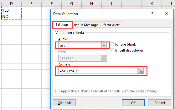
To create a drop-down list in column B (the control column):
- Select the cells in column B where you want a drop-down menu.
- Click Data > Data Validation.
- In the Data Validation dialog, choose List from the Allow dropdown. In the Source box, type or select a cell range containing the allowed values (e.g., YES,NO).

Now, you have a drop-down list in each cell of column B, allowing users to pick from set options: 
Repeat the Conditional Formatting setup as above, using a formula that matches the item you wish to trigger the grey formatting (e.g., =B2="YES"). After applying conditional formatting, your target cells in column A will automatically grey out whenever "YES" is selected in column B's dropdown. 
Additional tips and precautions:
- Make sure your conditional formatting range in column A matches the data area and aligns with column B's references. If they fall out of sync, formatting may not apply as expected.
- When copying or filling data in columns, check that references (e.g., B2) update appropriately.
- For best results, clear any old formatting from your ranges before applying new rules.
- To remove the greyed-out effect, either change the rule's trigger value in column B or delete the conditional formatting rule.
- If your worksheet is shared, ensure users know which values will trigger the format.
If conditional formatting is not working as expected, check that the cells in column B contain exactly the values the formula is testing (no extra spaces, correct case if not using exact match, and validation against hidden characters).

Unlock Excel Magic with Kutools AI
- Smart Execution: Perform cell operations, analyze data, and create charts—all driven by simple commands.
- Custom Formulas: Generate tailored formulas to streamline your workflows.
- VBA Coding: Write and implement VBA code effortlessly.
- Formula Interpretation: Understand complex formulas with ease.
- Text Translation: Break language barriers within your spreadsheets.
VBA: Automate greying out cells based on another column or drop-down list
For more advanced scenarios, such as batch-applying the formatting, handling multiple and more complex conditions, or when conditional formatting's rules and limit do not meet your requirements, you can use VBA code to automate the greying out of cells.
Common use cases:
- Automatically grey out entire rows or specific ranges based on drop-down selections or any logic tied to another column.
- Ensuring formatting remains consistent even after data imports or macro-driven sheet updates.
- Applying multiple conditional states that exceed built-in conditional formatting limits.
1. Click Developer Tools > Visual Basic to open the VBA editor (Alt+F11 is a shortcut). In the VBA window, click Insert > Module. Into the new module, copy and paste the following code:
Sub GreyOutCellsBasedOnAnotherColumn()
    Dim ws As Worksheet
    Dim lastRow As Long
    Dim checkCol As String
    Dim dataCol As String
    Dim i As Long
    Dim triggerValue As String

    On Error Resume Next
    xTitleId = "KutoolsforExcel"

    '----- Set parameters here -----
    Set ws = ActiveSheet ' Or: Set ws = ThisWorkbook.Sheets("Sheet1")
    checkCol = "B" ' Column to check (e.g., B)
    dataCol = "A" ' Column to grey out (e.g., A)
    triggerValue = "YES" ' Value that triggers grey out. Change as needed: "YES", "Complete", etc.

    '----- Find last row in the check column -----
    lastRow = ws.Cells(ws.Rows.Count, checkCol).End(xlUp).Row

    For i = 2 To lastRow ' Assumes header in row 1
        If ws.Cells(i, checkCol).Value = triggerValue Then
            ws.Cells(i, dataCol).Interior.Color = RGB(191, 191, 191) ' Grey fill
        Else
            ws.Cells(i, dataCol).Interior.ColorIndex = xlNone ' Remove fill if condition not met
        End If
    Next i
End Sub
2. To run the macro, press F5 with the code window active. The macro loops through each row in your worksheet—starting at row2 (so your first row can remain a header)—and checks column B for the trigger value (by default, "YES"). If it finds it, it fills the corresponding cell in column A with grey. If the trigger value is absent, any previous grey fill is removed (resetting the cell to default appearance).
You can customize the following parameters in the code:
- checkCol: Column to check (e.g., "B")
- dataCol: Column to grey out (e.g., "A")
- triggerValue: Value to match for grey fill (e.g., "YES", "Complete", any value in your list)
Cautions and tips:
- This macro changes cell backgrounds permanently. If you want colors to update live as you change data, consider re-running the macro after any update or use Worksheet_Change event scripting (advanced users only).
- The approach is not affected by the number of cells or conditional formatting rule limits, so it is ideal for large dynamic ranges or many conditions.
- If you mistakenly trigger the macro and want to remove grey fills, simply run it again after clearing or changing the relevant values.
- You can extend the If statement to add more conditions (e.g., greying out based on multiple choices, additional columns, or more complex logic).
Using VBA to manually or automatically grey out cells offers maximum flexibility for complex, large-scale, or highly tailored Excel solutions.
Best Office Productivity Tools
Supercharge Your Excel Skills with Kutools for Excel, and Experience Efficiency Like Never Before. Kutools for Excel Offers Over 300 Advanced Features to Boost Productivity and Save Time. Click Here to Get The Feature You Need The Most...
Office Tab Brings Tabbed interface to Office, and Make Your Work Much Easier
- Enable tabbed editing and reading in Word, Excel, PowerPoint, Publisher, Access, Visio and Project.
- Open and create multiple documents in new tabs of the same window, rather than in new windows.
- Increases your productivity by 50%, and reduces hundreds of mouse clicks for you every day!
All Kutools add-ins. One installer
Kutools for Office suite bundles add-ins for Excel, Word, Outlook & PowerPoint plus Office Tab Pro, which is ideal for teams working across Office apps.
- All-in-one suite — Excel, Word, Outlook & PowerPoint add-ins + Office Tab Pro
- One installer, one license — set up in minutes (MSI-ready)
- Works better together — streamlined productivity across Office apps
- 30-day full-featured trial — no registration, no credit card
- Best value — save vs buying individual add-in