How to transpose and link values in Excel?
In Excel, working with data often requires you to reorganize or present information in a different format. For instance, you may need to transpose a range - switching rows to columns or vice versa - and ensure that the transposed values remain linked to the original data so that any updates to the source are reflected instantly in the transposed set. By default, Excel allows you to paste copied data as links and also perform basic transpose operations, but combining both tasks into a single step is less straightforward. This article introduces several approaches to transpose and link values efficiently, with step-by-step instructions and practical tips.
Transpose and link pasted values by Name and formula
Transpose and link by Find and Replace function
Transpose and link using VBA macro for dynamic updates
 Transpose and link pasted values by Name and formula
This method allows you to transpose a group of values and keep them dynamically linked with the original data. By using a named range and a formula, any changes you make to the source data will be instantly reflected in the transposed group.
1. Select the data range you intend to transpose and link. In the Name box (next to the formula bar), type a descriptive name for this range (e.g., SPORT), and press Enter. Naming helps reference the range easily throughout the workbook.
2. If you’re using Excel 365, Excel 2021, or newer versions, select a single cell where you want the transposed data to start, enter the formula =TRANSPOSE(SPORT) (replace "SPORT" with your range name), and press Enter. Excel will automatically distribute the transposed data across multiple cells.
If you’re using Excel 2019 and earlier versions, highlight the target cells where you want the transposed and linked data displayed, type the same formula, and press Shift + Ctrl + Enter to create an array formula.

Your transposed data will appear and will stay synchronized with the original. Whenever the data in the named range is changed, the transposed display updates automatically.
Tips and precautions:
- In Excel 2019 and earlier, array formulas require selecting a range that matches the output shape. For example, if your source data has 5 rows, select 5 columns before entering the formula.
- Named ranges make formulas easier and more reliable - avoid using generic names and double-check spelling.
- If you need to expand the original data range later, you must update the named range reference accordingly for the transposed area to capture new data.
- If you see errors (#VALUE!), double-check cell selection and ensure you complete the formula with Shift + Ctrl + Enter, not just Enter.
Transpose and link by Find and Replace function
This technique utilizes Excel's Find and Replace function along with Paste Special options to achieve both transposing and linking. While somewhat indirect, it is useful when array formulas are not ideal, or for users preferring menu-driven steps.
1. Highlight your original data range. Press Ctrl + C to copy. Right-click the cell where you want to place the data, and from the Paste Special submenu, choose Link. This step pastes references instead of static values.
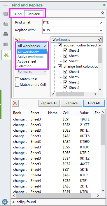
2. Now, open the Find and Replace dialog by pressing Ctrl + H. In the Find what box, enter = and in the Replace with box, type #=. This temporarily changes formulas to prevent issues with transposing later.
3. Click Replace All. You’ll see a dialog showing how many replacements were made. Click OK, then Close.
4. Copy the modified range by pressing Ctrl + C again. Right-click at your target destination, select Paste Special and then Transpose. This switches the orientation for you.
5. With the transposed data still selected, open Find and Replace again (Ctrl + H). In Find what, type #=; in Replace with, enter = to restore active links.
6. Choose Replace All once more, confirm the dialog, and close out. Your values are now transposed and remain linked to the original inputs.
Tips and precautions:
- Ensure you replace all equal signs before transposing, or you may get formula errors.
- After the steps, double-check that the transposed values change when you adjust original data, confirming the link is active.
- If you encounter formula errors, verify both your Find and Replace actions and your cell selections.
Transpose and link using VBA macro for dynamic updates
For users who need a scalable, automated solution - such as when the linked and transposed data spans a large range, or where frequent updates are required - a VBA macro can be used to dynamically generate transposed links. This approach is particularly useful in large or frequently edited sheets where manual methods are time-consuming, and where you want the transposed area to always be up to date with the source data.
1. Go to the Developer tab and click Visual Basic to open the Microsoft Visual Basic for Applications editor. If the Developer tab isn’t visible, see this guide: Show the Developer tab in Excel.
2. In the VBA editor, click Insert > Module to create a new module. Then, paste the following code into the editor window:
Sub TransposeLinkDynamic()
    Dim SourceRange As Range
    Dim DestCell As Range
    Dim r As Long, c As Long
    Dim nRows As Long, nCols As Long

    On Error Resume Next
    xTitleId = "KutoolsforExcel"

    Set SourceRange = Application.InputBox("Select the range to transpose and link", xTitleId, "", Type:=8)
    Set DestCell = Application.InputBox("Select the top-left cell of transposed linked output", xTitleId, "", Type:=8)

    nRows = SourceRange.Rows.Count
    nCols = SourceRange.Columns.Count

    For r = 1 To nCols
        For c = 1 To nRows
            DestCell.Offset(r - 1, c - 1).Formula = "=" & SourceRange.Cells(c, r).Address(ReferenceStyle:=xlA1, External:=True)
        Next c
    Next r
End Sub
3. To run the macro, click the ![]() button, or press F5. You’ll first be prompted to select the source range to transpose. Then, choose the top-left cell of the output area, where the transposed and linked data will appear.
button, or press F5. You’ll first be prompted to select the source range to transpose. Then, choose the top-left cell of the output area, where the transposed and linked data will appear.
All data in the output area will contain formulas dynamically linked to the original range, but shown in transposed format. This means any updates you make to the original data range are immediately reflected in the linked transposed area, and you won’t need to redo the process.
Tips and precautions:
- All formulas are constructed dynamically-if you move or resize the source range, rerun the macro as needed.
- If you get permissions errors or cannot run macros, check that macro security is enabled for your workbook, and save as .xlsm format.
Best Office Productivity Tools
Supercharge Your Excel Skills with Kutools for Excel, and Experience Efficiency Like Never Before. Kutools for Excel Offers Over 300 Advanced Features to Boost Productivity and Save Time. Click Here to Get The Feature You Need The Most...
Office Tab Brings Tabbed interface to Office, and Make Your Work Much Easier
- Enable tabbed editing and reading in Word, Excel, PowerPoint, Publisher, Access, Visio and Project.
- Open and create multiple documents in new tabs of the same window, rather than in new windows.
- Increases your productivity by 50%, and reduces hundreds of mouse clicks for you every day!
All Kutools add-ins. One installer
Kutools for Office suite bundles add-ins for Excel, Word, Outlook & PowerPoint plus Office Tab Pro, which is ideal for teams working across Office apps.
- All-in-one suite — Excel, Word, Outlook & PowerPoint add-ins + Office Tab Pro
- One installer, one license — set up in minutes (MSI-ready)
- Works better together — streamlined productivity across Office apps
- 30-day full-featured trial — no registration, no credit card
- Best value — save vs buying individual add-in