How to display different text than the actual value in same cell?
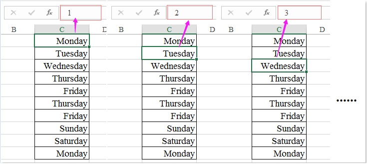
In Excel, the value you enter into a cell is typically shown both in the cell itself and in the formula bar, ensuring data consistency and transparency at all times. As illustrated in the first screenshot below, what appears in the cell matches exactly what you see in the formula bar. However, in certain scenarios—such as designing dashboards, creating reports, or presenting summarized information—you might wish to display text in a cell that differs from its underlying value. In this way, the cell could visually show descriptive text but retain its numeric or coded value in the formula bar, as shown in the second screenshot. Achieving this visual differentiation is useful for improving readability or conveying specific information, while still enabling calculations or data analysis using the underlying value. This article introduces practical methods to accomplish this in Excel, covering both built-in approaches and time-saving add-ins.

Display different text than the value in same cell with Conditional Formatting
Make the displayed text equal the actual value with Kutools for Excel
Alternative solution: Use VBA macro to dynamically display different texts
 Display different text than the value in same cell with Conditional Formatting
Suppose you aim to improve clarity in a summary table and make the content more intuitive. For instance, you want cell C1 to show the word "Monday," but its underlying value—the number that appears in the formula bar—remains 1. Similarly, C2 displays "Tuesday" while its actual value is 2, and so on. This technique is helpful when you want to present labels or friendly text while still relying on the original data for calculations, filtering, or referencing. Below is an example screenshot that demonstrates the effect:

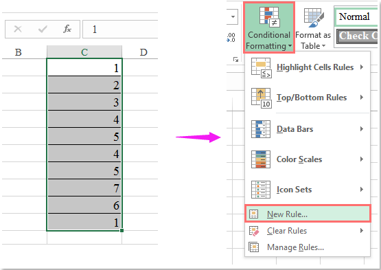
1. First, select the range of cells where you want to display alternate text (for example, cells C1 to C7). Then, on the ribbon, click Home > Conditional Formatting > New Rule. This opens the New Formatting Rule dialog box. Please see the screenshot below for visual reference:

2. In the New Formatting Rule window, select Use a formula to determine which cells to format from the list. In the formula field, enter the following formula (for instance, for C1 showing "Monday" when the value is 1):
=C1=1
Note: Replace C1 with the appropriate cell reference for your selection, and 1 with the actual value you want to conditionally change the display text for. If you are formatting a range (e.g., C1:C7), ensure that your formula starts with the top-left cell of your selection to apply the condition properly. If necessary, use relative or absolute references as appropriate. The dialog should look like this:

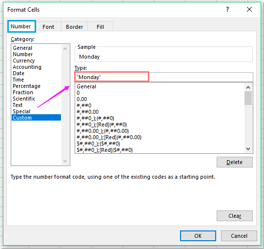
3. Click the Format button to open the Format Cells dialog box. Under the Number tab, select Custom in the left pane. In the Type field, type the text you wish to display, enclosed in double quotes—for example:
"Monday"
It is essential to use double quotes; otherwise, the cell may not display the text properly. See the example below:

Note: Make sure to include the quotes around your text, otherwise Excel will return an error or display the format code instead of your intended label.
4. Click OK to close the Format Cells dialog, then again click OK in the New Formatting Rule dialog to apply the rule. The targeted numeric values in the cells will now display as your specified text, such as “Monday” instead of 1, as illustrated below:

Note: To configure different values to show various texts, simply repeat the process for each value you want to customize. Enter the relevant formula in the Conditional Formatting dialog and specify the display text for each condition. This technique is efficient when dealing with a small fixed set of values such as days of the week, statuses, or categories.
| Conditional formula | Format (Number: Custom) |
| =C1=2 | "Tuesday" |
| =C1=3 | "Wednesday" |
| =C1=4 | "Thursday" |
| =C1=5 | "Friday" |
| =C1=6 | "Saturday" |
| =C1=7 | "Sunday" |
Applicable Scenario: This solution is ideal when you have a limited number of known values and want to present user-friendly labels while retaining their original values for calculations or lookups.
Advantages: No formulas or external code required; displays visually intuitive data.
Limitations: For each new value/text pair, a separate formatting rule must be added, which might get tedious for large data sets. The original cell value remains unchanged for calculation purposes, but the visible label can be misleading if not documented. Also, this approach does not physically change the cell value itself—only its display format changes conditionally.
Practical tips: If you need to reuse this display logic elsewhere, use the Format Painter tool to copy conditional formatting rules. If the rules seem not to work, double-check that the formula cell references match your selection exactly.
Troubleshooting: If the text does not appear as expected, verify there are no conflicting conditional formatting rules in the same cells. Also, ensure that your custom format string is entered in double quotes, and the formula references are correct. Note that Conditional Formatting only changes cell appearance and does not affect data exports or external system integration.
 Make the displayed text equal the actual value with Kutools for Excel
In some situations, after applying custom number formatting or conditional formatting, you may notice that the cell's displayed value no longer matches its true underlying value, leading to confusion or errors when performing further analysis or sharing data. If you want to quickly revert cells—so the text seen in the cell matches exactly what appears in the formula bar, and both reflect the actual stored value—Excel does not provide a straightforward native feature for this task.
With Kutools for Excel, resolving this issue is remarkably efficient. Its To Actual function is designed precisely for this purpose: to instantly synchronize display text with the real cell value, removing any custom formatting that causes mismatches.
Kutools for Excel - Packed with over 300 essential tools for Excel. Make Excel tasks faster, easier, and more efficient. Download now!
After installing Kutools for Excel, follow these simple steps:
1. Select the cells where you want the displayed text and actual value to match, then navigate to the Kutools tab and click To Actual. Refer to the screenshot for precise location:

2. In a single click, the display is updated and the displayed text is now consistent with the underlying data. The cell shows the real value as it appears in the formula bar:

Applicable Scenario: Use this method when you want to unmask custom-formatted cells and restore the display so it shows the literal values, preventing misinterpretation or data input errors.
Advantages: Extremely fast to use, batch processing is supported, and no need to manually clear individual formats.
Limitations: Requires installation of the Kutools for Excel add-in. Be careful when working in shared environments, as changes are immediate and affect the appearance of your data for all downstream uses.
Click to Download Kutools for Excel and free trial Now!
 Alternative solution: Use VBA macro to dynamically display different texts
If you require more dynamic mapping—such as handling values based on external lookups, user inputs, or large data sets—a custom VBA macro provides great flexibility. This solution is well-suited to advanced users and scenarios where native formatting is insufficient.
1. Press Alt+F11 to open the VBA editor. In the Microsoft Visual Basic for Applications window, click Insert > Module.
2. Copy and paste the following code into the module:
Sub DisplayCustomText()
    Dim cell As Range
    Dim WorkRng As Range
    On Error Resume Next
    xTitleId = "KutoolsforExcel"
    Set WorkRng = Application.Selection
    Set WorkRng = Application.InputBox("Select range for custom display", xTitleId, WorkRng.Address, Type:=8)
    For Each cell In WorkRng
        Select Case cell.Value
            Case 1
                cell.NumberFormat = """Monday"""
            Case 2
                cell.NumberFormat = """Tuesday"""
            Case 3
                cell.NumberFormat = """Wednesday"""
            Case 4
                cell.NumberFormat = """Thursday"""
            Case 5
                cell.NumberFormat = """Friday"""
            Case 6
                cell.NumberFormat = """Saturday"""
            Case 7
                cell.NumberFormat = """Sunday"""
            Case Else
                cell.NumberFormat = "General"
        End Select
    Next
End Sub3. Run the macro by clicking the ![]() button, or press F5. A dialog will appear prompting you to select the range where you want this logic applied.
button, or press F5. A dialog will appear prompting you to select the range where you want this logic applied.
After running, each cell in the selected range will display the day name associated with its value, without changing the underlying numeric value.
Parameter explanations:
The macro uses the NumberFormat property to set how values display, matching them to a day name if they are between 1 and 7; otherwise, the default format is applied.
Precautions: Results are visual only; actual cell values remain unchanged for formulas and calculations. To revert, manually reset the number format or use Kutools’ To Actual feature.
Tips: You may adapt this macro for other mapping schemes simply by editing the Select Case blocks.
Summary suggestions:
Choosing among Conditional Formatting, or the VBA approach depends on your specific needs—considering the number of different mappings, ease of later maintenance, compatibility with shared files, and user familiarity. For quick restoration or batch operations, Kutools for Excel offers highly convenient options to ensure data fidelity and clarity.
Best Office Productivity Tools
Supercharge Your Excel Skills with Kutools for Excel, and Experience Efficiency Like Never Before. Kutools for Excel Offers Over 300 Advanced Features to Boost Productivity and Save Time. Click Here to Get The Feature You Need The Most...
Office Tab Brings Tabbed interface to Office, and Make Your Work Much Easier
- Enable tabbed editing and reading in Word, Excel, PowerPoint, Publisher, Access, Visio and Project.
- Open and create multiple documents in new tabs of the same window, rather than in new windows.
- Increases your productivity by 50%, and reduces hundreds of mouse clicks for you every day!
All Kutools add-ins. One installer
Kutools for Office suite bundles add-ins for Excel, Word, Outlook & PowerPoint plus Office Tab Pro, which is ideal for teams working across Office apps.
- All-in-one suite — Excel, Word, Outlook & PowerPoint add-ins + Office Tab Pro
- One installer, one license — set up in minutes (MSI-ready)
- Works better together — streamlined productivity across Office apps
- 30-day full-featured trial — no registration, no credit card
- Best value — save vs buying individual add-in