How to calculate weighted average in an Excel Pivot Table?

Calculating the weighted average for data in Excel is a common requirement, especially when your data points contribute unequally to the final result. For straightforward ranges, the SUMPRODUCT and SUM functions offer a quick solution. However, when working with Pivot Tables, you might notice that calculated fields do not natively support these functions. This can complicate matters when you want to compute weighted averages directly within the Pivot Table. Understanding these limitations and learning alternative approaches can help you efficiently summarize your data in various scenarios. This article explores different ways to calculate a weighted average in a Pivot Table, covering both classic solutions and newer features available in Excel.

Calculate weighted average in an Excel Pivot Table
VBA Code - Automate Weighted Average Calculation in Pivot Table
Power Pivot (Data Model) - Use DAX to Calculate Weighted Average in Pivot Table

Calculate weighted average in an Excel Pivot Table

Power Pivot (Data Model) - Use DAX to Calculate Weighted Average in Pivot Table

With modern versions of Excel, the Power Pivot add-in (also known as the Data Model) unlocks new calculation options using DAX formulas (Data Analysis Expressions). This enables you to calculate weighted averages directly in the Pivot Table without creating extra helper columns in your underlying data.

Applicable scenarios: Ideal when working with large datasets or connected tables, and when you want calculations to refresh automatically with your data. This approach is especially useful for business analyses and dashboards where maintaining a clean source table is preferred.

Instructions:

1. Enable Power Pivot add-in
   Go to File > Options > Add-ins. In the Manage drop-down, select COM Add-ins, click Go, and check Power Pivot.
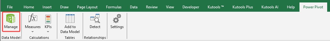
2. Add data to Power Pivot
   Select your table in the worksheet, then click Power Pivot > Manage to open the Power Pivot window.

   

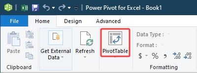
3. Create PivotTable from Power Pivot
   In the Power Pivot window, go to Home > PivotTable.

   

   Then choose where to insert it (e.g., Existing Worksheet) and click OK.

   

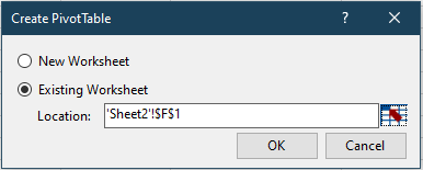
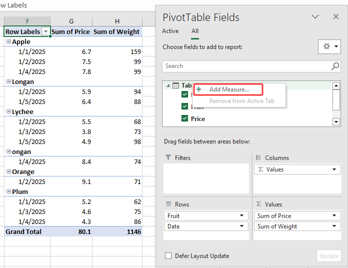
4. Build PivotTable and add a measure
   In the newly created PivotTable field list, drag fields to the appropriate areas. Then right-click the table name and select Add Measure.

   

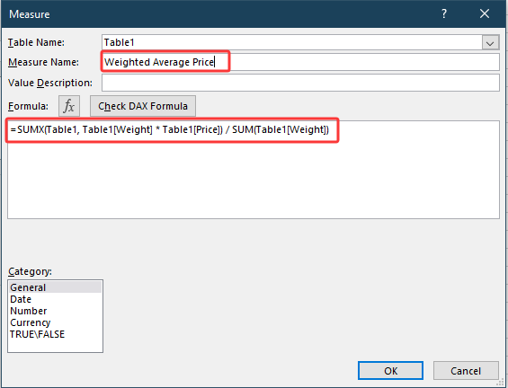
5. Define the measure
   In the Measure dialog box:
   1. Name the measure (e.g., Weighted Average Price).
   2. Enter the following DAX expression for weighted average.

      =SUMX(Table1, Table1[Weight] * Table1[Price]) / SUM(Table1[Weight])

      (Replace Table1, [Weight], and [Price] with your actual table and field names.)
   3. Click OK to add it.

      

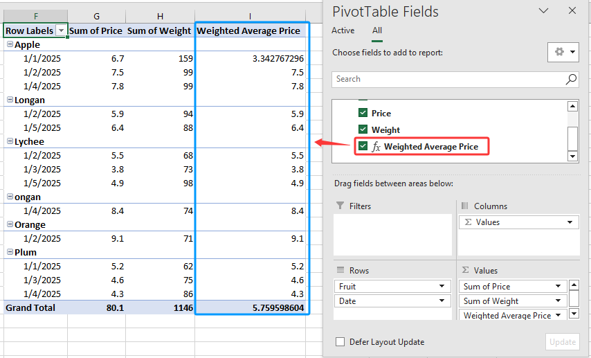
6. Use the measure in PivotTable
   The newly added measure will appear in the field list and can be dragged into the Values area like any other field.

   

Tips and troubleshooting:
- DAX formulas are case-insensitive but field/table names must match your model.
- Changing underlying data refreshes the measure automatically in your Pivot Table.
- If you get blank or unexpected results, check for zero or missing weight values and make sure your data model refreshes properly.

Pros: No modifications needed in source data; calculations update instantly with data changes and allow advanced summarizations.
Cons: Power Pivot is not available in all Excel editions and may require initial setup; users unfamiliar with DAX may face a learning curve.

Unlock Excel Magic with Kutools AI

• Smart Execution: Perform cell operations, analyze data, and create charts—all driven by simple commands.
• Custom Formulas: Generate tailored formulas to streamline your workflows.
• VBA Coding: Write and implement VBA code effortlessly.
• Formula Interpretation: Understand complex formulas with ease.
• Text Translation: Break language barriers within your spreadsheets.

Enhance your Excel capabilities with AI-powered tools. Download Now and experience efficiency like never before!

Related articles: