How to populate rows based on specified cell value in Excel?
Supposing you have a project table with corresponding person’s name who is in charge of each project as below screenshot shown. And now you need to list out all project names in rows based on given person, how to achieve it? Actually an array formula in this article can help you solve the problem.

Populate rows based on specified cell value with array formula
Populate rows based on specified cell value with array formula
Please do as follows to populate rows with the corresponding record based on given value in Excel.
1. Select a blank cell, enter the below formula into it and then press the Ctrl + Shift + Enter keys.
=IFERROR(INDEX(Sheet2!A$1:A$10,SMALL(IF(Sheet2!B$1:B$10=D$2,ROW(A$1:A$10)),ROWS(D$2:D2))),"")

Note: in the formula, Sheet2 is the name of current worksheet, A$1:A$10 is the column range contains all project names (include header), B$1:B$10 is the column range contains all person names (include header), and D$2 is the cell contains the person name you will populate rows based on. Please change them as you need.
2. Select the first result cell, drag the Fill Handle down to fill all rows with corresponding task names. See screenshot:
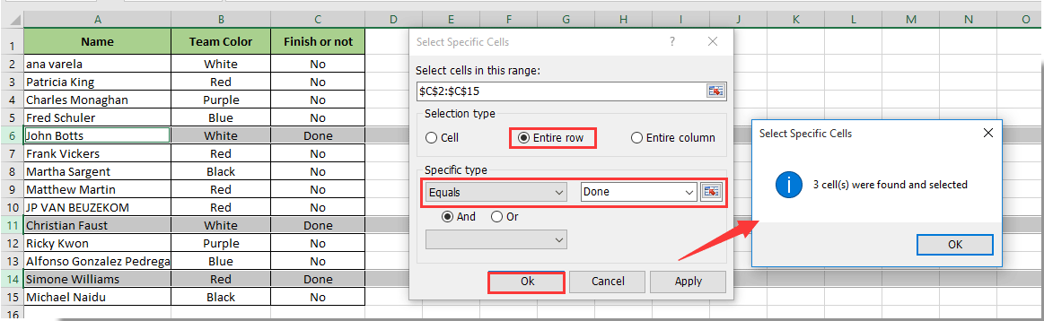
Easily select entire rows based on cell value in a certian column:
The Select Specific Cells utility of Kutools for Excel can help you quickly select entire rows based on cell value in a certian column in Excel as below screenshot shown. After selecting all rows based on cell value, you can manually move or copy them to a new location as you need.
Download and try it now! (30-day free trail)
Related articles:
- How to move entire row to another sheet based on cell value in Excel?
- How to lock or unlock cells based on values in another cell in Excel?
Best Office Productivity Tools
Supercharge Your Excel Skills with Kutools for Excel, and Experience Efficiency Like Never Before. Kutools for Excel Offers Over 300 Advanced Features to Boost Productivity and Save Time. Click Here to Get The Feature You Need The Most...
Office Tab Brings Tabbed interface to Office, and Make Your Work Much Easier
- Enable tabbed editing and reading in Word, Excel, PowerPoint, Publisher, Access, Visio and Project.
- Open and create multiple documents in new tabs of the same window, rather than in new windows.
- Increases your productivity by 50%, and reduces hundreds of mouse clicks for you every day!
All Kutools add-ins. One installer
Kutools for Office suite bundles add-ins for Excel, Word, Outlook & PowerPoint plus Office Tab Pro, which is ideal for teams working across Office apps.
- All-in-one suite — Excel, Word, Outlook & PowerPoint add-ins + Office Tab Pro
- One installer, one license — set up in minutes (MSI-ready)
- Works better together — streamlined productivity across Office apps
- 30-day full-featured trial — no registration, no credit card
- Best value — save vs buying individual add-in