How to VLOOKUP then multiply in Excel tables?
In day-to-day business or data analysis scenarios, it's common to encounter situations where you need to extract information from structured tables and perform further calculations based on lookup results. For example, you might have a rule table that defines different profit rates depending on the sales volume of products, and another table that records the actual sales volumes for each product. The challenge lies in efficiently determining the applicable profit rate for each product according to its actual sales, and then calculating the profit by multiplying the real sales value by the appropriate profit rate. This approach is particularly useful when pricing strategies or bonuses depend on variable thresholds or rules, making it essential for sales, finance, or inventory management tasks.
Lookup then multiple based on criteria
Lookup then multiply based on criteria
To accomplish this task, you can use Excel's VLOOKUP function in combination with MATCH, or leverage the INDEX function for similar results. Each solution has its use cases and subtle differences, allowing you to choose the most suitable method for your data structure and preferences. Both approaches help retrieve the relevant profit rate based on the combination of product and sales volume, then calculate the actual profit amount efficiently.
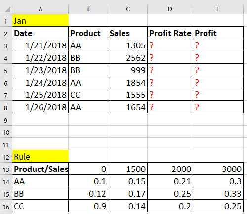
Select the cell immediately to the right of your product’s real sales amount. Next, enter the following formula to extract the matching profit rate:
=VLOOKUP(B3,$A$14:$E$16,MATCH(C3,$A$13:$E$13),0)After typing the formula, press Enter to display the profit rate that corresponds to both the product and its sales volume. To automatically calculate the profit rates for all the products, use the fill handle (small square at the lower right of the cell) to drag the formula down through all relevant rows in your list.
In this formula:
- B3: Product name or identifier to look up (criterion 1)
- C3: Actual sales value or category (criterion 2)
- $A$14:$E$16: Range containing the rule table (products and corresponding profit rates)
- $A$13:$E$13: Header row that contains sales ranges or categories
It's important to ensure that the lookup ranges ($A$14:$E$16 and $A$13:$E$13) are set as absolute references by using $. This prevents errors when copying the formulas to other rows. If the headers or product names in your tables contain extra spaces or inconsistent formatting, use the TRIM or CLEAN function to standardize your data before applying the formulas. Be attentive to data types—categorical and numerical mismatches in your criteria cells (B3, C3) and header row/columns could lead to lookup errors or unintended results.
Once the profit rates are returned, calculate the profit for each product by multiplying the obtained profit rate by the relevant actual sales. In the next adjacent column, enter this formula:
=D3*C3Here, D3 contains the profit rate calculated above, and C3 is the actual sales figure. Press Enter, and use the fill handle to drag the formula down for all other products, thereby calculating each one’s profit with ease.
Tip: If you're working with a large dataset or need a more flexible approach, you can also use the INDEX and MATCH combination for your lookup. This is especially beneficial if your lookup table isn't structured with the lookup column on the left as required by VLOOKUP, or if you prefer referencing columns and rows separately. For example, enter the following formula to get the profit rate based on both product and sales:
=INDEX($B$14:$E$16,MATCH(B3,$A$14:$A$16,0),MATCH(C3,$B$13:$E$13))In this formula:
- $B$14:$E$16: Range containing only the profit rates.
- MATCH(B3,$A$14:$A$16,0): Finds the row number matching the target product.
- MATCH(C3,$B$13:$E$13): Finds the column number corresponding to the sales amount or category.
After entering the formula, press Enter, and use the fill handle to apply it to the rest of your table as needed. INDEX and MATCH are generally less prone to errors if the structure of your lookup table is more complex or changes in the future, offering more versatility.
If you encounter #N/A or #REF! errors, double check that your lookup arguments are spelled correctly, the ranges match your data's actual layout, and the sales category values are consistent between tables. It's best to keep your criterion values standardized and avoid hidden spaces or unexpected formatting in your datasets.
Alternative formulas such as XLOOKUP or SUMPRODUCT can also be considered if you are using newer versions of Excel or need more advanced array or multi-condition matching. For example, XLOOKUP allows for easier syntax and more intuitive error handling compared to VLOOKUP.
After finalizing your profit calculations, consider cross-checking a few results manually to ensure that the lookup rules and calculations apply as expected. This can help catch inconsistencies due to table structure or entry errors. Keeping lookup table ranges updated with data changes will also help maintain accuracy over time.
Best Office Productivity Tools
Supercharge Your Excel Skills with Kutools for Excel, and Experience Efficiency Like Never Before. Kutools for Excel Offers Over 300 Advanced Features to Boost Productivity and Save Time. Click Here to Get The Feature You Need The Most...
Office Tab Brings Tabbed interface to Office, and Make Your Work Much Easier
- Enable tabbed editing and reading in Word, Excel, PowerPoint, Publisher, Access, Visio and Project.
- Open and create multiple documents in new tabs of the same window, rather than in new windows.
- Increases your productivity by 50%, and reduces hundreds of mouse clicks for you every day!
All Kutools add-ins. One installer
Kutools for Office suite bundles add-ins for Excel, Word, Outlook & PowerPoint plus Office Tab Pro, which is ideal for teams working across Office apps.
- All-in-one suite — Excel, Word, Outlook & PowerPoint add-ins + Office Tab Pro
- One installer, one license — set up in minutes (MSI-ready)
- Works better together — streamlined productivity across Office apps
- 30-day full-featured trial — no registration, no credit card
- Best value — save vs buying individual add-in