How to vlookup and return background color along with the lookup value in Excel?
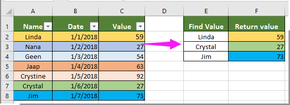
Supposing you have a table as below screenshot shown. Now you want to check if a specified value is in column A and then return the corresponding value along with its background color in column C. How to achieve it? The method in the article can help you solve the problem.
Vlookup and return background color with lookup value by User-defined function
Vlookup and return background color with lookup value by User-defined function
Please do as follows to lookup a value and return its corresponding value along with background color in Excel.
1. In the worksheet contains the value you want to vlookup, right-click the sheet tab and select View Code from the context menu. See screenshot:

2. In the opening Microsoft Visual Basic for Applications window, please copy below VBA code into the Code window.
VBA code 1: Vlookup and return background color with the lookup value
Sub Worksheet_Change(ByVal Target As Range)
    Dim I As Long
    Dim xKeys As Long
    Dim xDicStr As String
    On Error Resume Next
    Application.ScreenUpdating = False
    xKeys = UBound(xDic.Keys)
    If xKeys >= 0 Then
        For I = 0 To UBound(xDic.Keys)
            xDicStr = xDic.Items(I)
            If xDicStr <> "" Then
                Range(xDic.Keys(I)).Interior.Color = _
                Range(xDic.Items(I)).Interior.Color
            Else
                Range(xDic.Keys(I)).Interior.Color = xlNone
            End If
        Next
        Set xDic = Nothing
    End If
    Application.ScreenUpdating = True
End Sub
3. Then click Insert > Module, and copy the below VBA code 2 into the Module window.
VBA code 2: Vlookup and return background color with the lookup value
Public xDic As New Dictionary
Function LookupKeepColor (ByRef FndValue, ByRef LookupRng As Range, ByRef xCol As Long)
    Dim xFindCell As Range
    On Error Resume Next
    Set xFindCell = LookupRng.Find(FndValue, , xlValues, xlWhole)
    If xFindCell Is Nothing Then
        LookupKeepColor = ""
        xDic.Add Application.Caller.Address, ""
    Else
        LookupKeepColor = xFindCell.Offset(0, xCol - 1).Value
        xDic.Add Application.Caller.Address, xFindCell.Offset(0, xCol - 1).Address
    End If
End Function
4. After inserting the two codes, then click Tools > References. Then check the Microsoft Script Runtime box in the References – VBAProject dialog box. See screenshot:

5. Press the Alt + Q keys to exit the Microsoft Visual Basic for Applications window and go back to the worksheet.
6. Select a blank cell adjacent to the lookup value, and then enter formula =LookupKeepColor(E2,$A$1:$C$8,3) into the Formula Bar, and then press the Enter key.

Note: In the formula, E2 contains the value you will lookup, $A$1:$C$8 is the table range, and number 3means that the corresponding value you will return locates in the third column of the table. Please change them as you need.
7. Keep selecting the first result cell, and drag the Fill Handle down to get all results along with their background color. See screenshot.

Related articles:
- How to copy source formatting of the lookup cell when using Vlookup in Excel?
- How to vlookup and return date format instead of number in Excel?
- How to use vlookup and sum in Excel?
- How to vlookup return value in adjacent or next cell in Excel?
- How to vlookup value and return true or false / yes or no in Excel?
Best Office Productivity Tools
Supercharge Your Excel Skills with Kutools for Excel, and Experience Efficiency Like Never Before. Kutools for Excel Offers Over 300 Advanced Features to Boost Productivity and Save Time. Click Here to Get The Feature You Need The Most...
Office Tab Brings Tabbed interface to Office, and Make Your Work Much Easier
- Enable tabbed editing and reading in Word, Excel, PowerPoint, Publisher, Access, Visio and Project.
- Open and create multiple documents in new tabs of the same window, rather than in new windows.
- Increases your productivity by 50%, and reduces hundreds of mouse clicks for you every day!
All Kutools add-ins. One installer
Kutools for Office suite bundles add-ins for Excel, Word, Outlook & PowerPoint plus Office Tab Pro, which is ideal for teams working across Office apps.
- All-in-one suite — Excel, Word, Outlook & PowerPoint add-ins + Office Tab Pro
- One installer, one license — set up in minutes (MSI-ready)
- Works better together — streamlined productivity across Office apps
- 30-day full-featured trial — no registration, no credit card
- Best value — save vs buying individual add-in