How to reverse the order of items in an Excel chart legend?
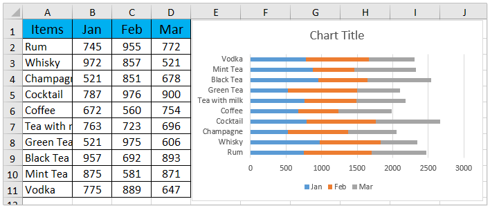
When working with complex datasets, visualizing information through charts in Excel is a common practice and helps in the effective communication of data patterns. For instance, suppose you have a sales table listing monthly sales data, and you have illustrated this information by creating a stacked bar chart as shown in the screenshot below. By default, Excel will display the legend starting with the first entry of your data—such as January sales—then followed by February, and so forth, often matching the data’s chronological order. However, certain reporting requirements or better visual comparisons might call for reversing this sequence—for example, listing March first and January last in both the chart and its legend. Understanding how to reverse the order of items in a chart legend allows you to tailor your reports to meet specific needs or presentation preferences. This tutorial provides detailed step-by-step instructions for reversing legend item order in stacked bar charts in Excel.
Reverse the order of items in an Excel chart legend

Reverse the order of items in an Excel chart legend
If you want to reverse the display order of legend items in a stacked bar chart directly in Excel, you can do this by managing the data series’ arrangement. Changing legend order is helpful for customizing the visualization to match reporting priorities or for consistency with other business documents. Here’s how you can manually rearrange legend items from top to bottom:
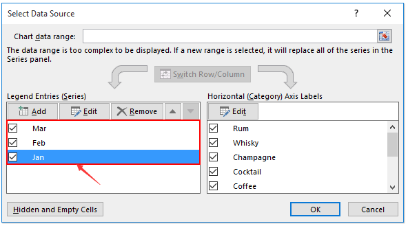
1. Right-click anywhere on the chart and select Select Data from the context menu. This opens the Select Data Source dialog box, where all your chart series are listed.
2. In the dialog box, focus on the Legend Entries (Series) section. Click to highlight your first legend item—for example, Jan—and then use the Move Down button ![]() to send it to the bottom of the series list.
to send it to the bottom of the series list. 
3. Repeat the process as needed: move each remaining series down until the original last series appears at the top of the list. When series are reordered here, their legend positions update instantly. When finished, click OK to confirm and close the dialog box.
Upon returning to your worksheet, you will see that the chart legend now displays the items in reverse order. 
Tips:
- If your chart contains many series, keep track of series labels to avoid confusion during reordering. Consider writing down the initial order before making changes.
- Manually rearranging requires careful attention if you later add or remove series. Check the legend order after any changes to make sure it remains as intended.
- If the chart is linked to a dynamic range or is regularly updated, you may need to repeat this process after updating the source data.
Troubleshooting:
- If the Move Up/Move Down buttons are unavailable or greyed out, try clicking directly on the series name in the list before using the buttons.
- If changes don't appear in the chart, try closing and reopening the file or pressing F9 to refresh.
Related articles:
Best Office Productivity Tools
Supercharge Your Excel Skills with Kutools for Excel, and Experience Efficiency Like Never Before. Kutools for Excel Offers Over 300 Advanced Features to Boost Productivity and Save Time. Click Here to Get The Feature You Need The Most...
Office Tab Brings Tabbed interface to Office, and Make Your Work Much Easier
- Enable tabbed editing and reading in Word, Excel, PowerPoint, Publisher, Access, Visio and Project.
- Open and create multiple documents in new tabs of the same window, rather than in new windows.
- Increases your productivity by 50%, and reduces hundreds of mouse clicks for you every day!
All Kutools add-ins. One installer
Kutools for Office suite bundles add-ins for Excel, Word, Outlook & PowerPoint plus Office Tab Pro, which is ideal for teams working across Office apps.
- All-in-one suite — Excel, Word, Outlook & PowerPoint add-ins + Office Tab Pro
- One installer, one license — set up in minutes (MSI-ready)
- Works better together — streamlined productivity across Office apps
- 30-day full-featured trial — no registration, no credit card
- Best value — save vs buying individual add-in