If you want to create a YES or NO drop down list with color in Excel, please do as follows:

1. Select the list you will fill with the YES or NO drop down list, and click Data > Data Validation > Data Validation. See screenshot:

2. In the Data Validation dialog, under the Settings tab, please select List from the Allow drop down list, type Yes,No in the Source box, and click the OK button. See screenshot:

Now you have added a YES or NO drop down list in the selected list. Please go ahead to add color for the drop down list.

3. Select the table without header row, and click Home > Conditional Formatting > New Rule. See screenshot:

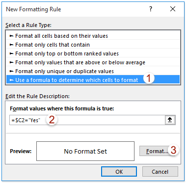
4. In the New Formatting Rule dialog, please (1) click to highlight the Use a formula to determine which cells to format option in the Select a Rule Type list box; (2) type =$C2="Yes" in the Format values where this formula is true box, and (3) click the Format button. See screenshot:
Note: In the formula =$C2="Yes", $C2 is the first cell with YES or NO drop down list, and you can change it as you need.

5. In the Format Cells dialog, please enable the Fill tab, specify a background color, and click the OK button successively to close both dialogs.

Now when you click the cells in the specified list, it will pop out the YES or NO drop down list. And when you select Yes from the drop down list, it will automatically highlight the entire row with the specified color. See screenshot:

Note: If you have installed Kutools for Excel, you can apply its Auto Save feature to save the range with data validation and conditional formatting as an AutoText entry, and then reuse it with clicks only. Get it Now!

Here in the second method, I will introduce the Colored Drop-down List feature of Kutools for Excel, which can help you quickly apply conditional formatting and highlight cells or rows based on the drop-down list selections easily.

1. Select the list you will fill with the YES or NO drop-down list, and click click Kutools > Drop-down List > Colored Drop-down List to enable this feature.

2. In the popping out Kutools for Excel dialog, please click Yes, please help me to create option to go ahead.
Tips: If you have added the YES or NO drop-down list for the selection, please click the No, I know the Data Validation feature, and then jump to the Step 4.

3. In the Create simple drop down list dialog box, please check if the selection range is added in the Apply to section, type YES,NO in the Source box, and click the Ok button.

4. In the Colored Drop-down list dialog, please do as follows:
(1) Check the Row of data range option in the Apply to section;
(2) In the Data validation (Drop-down List) Range box, normally the selected column containing the Yes and No drop-down list is entered here. And you can reselect or change it as you need.
(3) In the Highlight rows box, please select the rows matched with the specified data validation range;
(4) In the List Items section, please select one of drop-down list selection, says Yes, and click to highlight a color in the Select color section. And repeat this operation to assign colors for other drop-down list selections.

5. Click the Ok button.

From now on, the rows will be highlighted or unhighlighted automatically based on the selections of the drop-down list. See screenshot:

Kutools for Excel includes more than 300 handy tools for Excel, free to try without limitation in 30 days. Free Trial Now!      Buy Now!