How to filter data by multiple conditions in Google sheets?
In daily work, it is common to deal with large datasets and the need to quickly extract data that meets specific criteria. For instance, you may want to review sales records for specific products, filter out rows where certain conditions are met, or analyze data that matches a combination of requirements. In Microsoft Excel, the Advanced Filter feature is frequently used for these multi-condition filtering tasks. However, Google Sheets does not provide a direct counterpart to Advanced Filter, making such filtering seem challenging at first glance.
This article demonstrates several practical methods for achieving multi-condition filtering in Google Sheets, all using built-in formulas. By mastering these methods, you can efficiently analyze and present data according to your needs, even without advanced tools. You’ll also find guidance on troubleshooting common formula issues, and alternative ways to accomplish similar results when complex filtering is needed.
Filter data by multiple conditions in one column with formula
Filter data by multiple conditions in multiple columns with formula
Alternative solutions: Filter function with OR/AND logic, Filter Views in Google Sheets
Filter data by multiple conditions in one column with formula
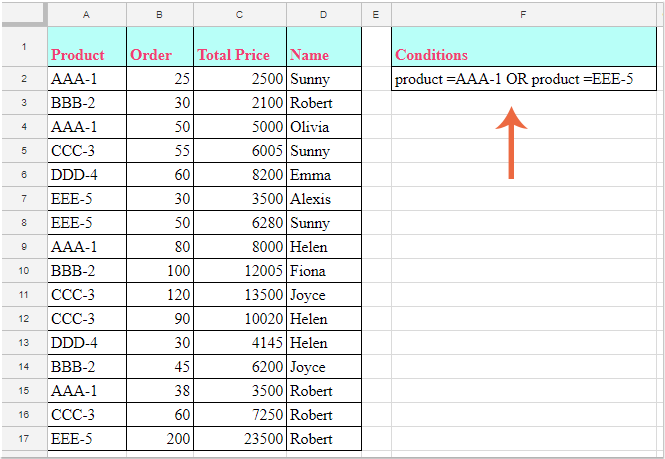
Suppose you want to extract all rows in a dataset where the value in column A is either "AAA-1" or "EEE-5". This requirement is very common—such as when tracking specific product SKUs or isolating data for targeted reporting in Google Sheets.

To perform this task, you can use the FILTER function with multiple conditions connected, which acts similarly to the OR logical operator. Please do the following:
Enter the following formula in a blank cell where you wish to display the filtered results:
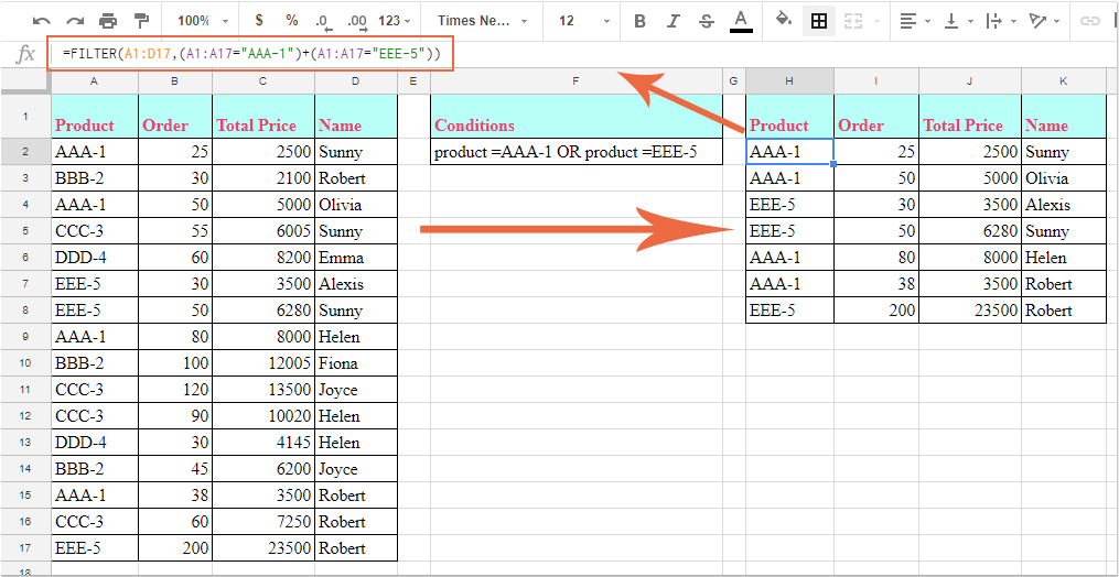
=FILTER(A1:D17, (A1:A17="AAA-1") + (A1:A17="EEE-5"))After typing the formula, simply press the Enter key. Google Sheets will instantly return all rows where the product in column A is either "AAA-1" or "EEE-5", as illustrated in the screenshot below:

Notes and tips:
1. In the formula above:
- A1:D17 represents the entire data range you wish to filter.
- A1:A17 is the specific column in which you apply your conditions.
- "AAA-1" and "EEE-5" are the filter criteria—replace these with your desired values as required for your dataset.
2. To add more filtering conditions, expand the formula by adding additional conditions with + to represent the OR logic. For example:
=FILTER(Range, (Condition1) + (Condition2) + (Condition3) + ...)Each added condition is enclosed in parentheses and separated by a plus sign. This construction lets Google Sheets filter the data to display rows that match any of the listed conditions in the target column.
3. Double-check that the ranges in your FILTER formula match in size. If the condition range is shorter than the data range, some matching results may be excluded.
4. The FILTER function is dynamic—if your source data updates, the filtered results will update automatically.
If you receive a #N/A error, it usually means no rows meet your conditions.
Filter data by multiple conditions in multiple columns with formula
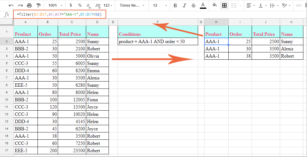
In many cases, you may need more granularity—for example, listing all rows where the product is "AAA-1" and the order quantity is less than 50. Combining criteria from multiple columns provides more precise filtering, often needed in business scenarios like inventory reviews or selective reporting.

To accomplish this, use the FILTER function and separate each condition with a comma, which acts as an AND logical operator. Please enter this formula into a blank cell where you want the results to appear:
=FILTER(A1:D17, A1:A17="AAA-1", B1:B17<50)After pressing Enter, Google Sheets immediately outputs all rows where both conditions are satisfied. Check the sample screenshot below to see the outcome:

Notes and tips:
1. In the formula:
- A1:D17: The data range to filter.
- A1:A17="AAA-1": First condition applied to the product column.
- B1:B17<50: Second condition applies to another column (e.g., order quantity).
You can customize conditions and ranges to match your sheet—just ensure all ranges have the same row count.
2. To filter by more than two conditions (across different columns), add extra conditions, separated by commas, to the FILTER formula. For example:
=FILTER(Range, Condition1, Condition2, Condition3, ...)Each additional condition refines the filter; all must be satisfied (logical AND relationship) for a row to be included.
3. Double-check comparison operators for numerical/ date criteria (<, >, <=, >=, etc.) and quotation marks for text (e.g., "ProductName"), to avoid formula errors.
4. The FILTER formula in Google Sheets recalculates automatically when your source data changes, keeping the results up to date without manual refreshes.
If the formula returns an error, verify that all ranges are of equal length, and that no referenced cells contain invalid data (like text in a numeric column for a comparison).
Alternative solutions for filtering data by multiple conditions in Google Sheets
In addition to the main FILTER function approaches, there are other methods and enhancements you may find useful for more complex scenarios:
Filter function with custom OR/AND logic using ARRAYFORMULA and REGEXMATCH
When you need to check for multiple text values (e.g., several keywords), REGEXMATCH lets you specify a pattern:
1. In a blank cell, enter the following formula to extract rows where column A matches "AAA-1", "EEE-5", or "CCC-2":
=FILTER(A1:D17, ARRAYFORMULA(REGEXMATCH(A1:A17, "AAA-1|EEE-5|CCC-2")))This formula uses REGEXMATCH to look for any occurrence of the listed values in column A. Adjust the pattern as needed, separating alternative values with | (pipe).
2. After inputting the formula, press Enter to see all rows matching any of the specified items. This is particularly useful for flexible textual filters that may grow over time.
Using Filter Views for interactive multi-condition filtering
For those who want a user-friendly, no-formula approach, Google Sheets provides Filter Views and the standard Filter, which allow you to create temporary or saved filters without altering the underlying data. This is especially useful if you need to share filtered results without removing or hiding data for others.
Tip:
- Select your data range (including headers), then click the Filter button in the toolbar, or go to Data > Create a filter.
- Click the filter icon in a column header to select specific values or set number/text criteria.
When working with any of these filtering techniques in Google Sheets:
- Be sure to carefully align ranges in your formulas to avoid errors.
- Update conditions and references as your data structure changes.
- If your filtered results show unexpected output, re-examine each criteria and operator, and confirm there are no hidden characters (e.g., extra spaces) in your data.
Using these methods, you can address nearly any filtering requirement in Google Sheets efficiently. If you encounter persistent issues or have especially complex, repetitive filtering tasks, consider creating custom Apps Script functions, or explore available add-ons for Google Sheets.
Best Office Productivity Tools
Supercharge Your Excel Skills with Kutools for Excel, and Experience Efficiency Like Never Before. Kutools for Excel Offers Over 300 Advanced Features to Boost Productivity and Save Time. Click Here to Get The Feature You Need The Most...
Office Tab Brings Tabbed interface to Office, and Make Your Work Much Easier
- Enable tabbed editing and reading in Word, Excel, PowerPoint, Publisher, Access, Visio and Project.
- Open and create multiple documents in new tabs of the same window, rather than in new windows.
- Increases your productivity by 50%, and reduces hundreds of mouse clicks for you every day!
All Kutools add-ins. One installer
Kutools for Office suite bundles add-ins for Excel, Word, Outlook & PowerPoint plus Office Tab Pro, which is ideal for teams working across Office apps.
- All-in-one suite — Excel, Word, Outlook & PowerPoint add-ins + Office Tab Pro
- One installer, one license — set up in minutes (MSI-ready)
- Works better together — streamlined productivity across Office apps
- 30-day full-featured trial — no registration, no credit card
- Best value — save vs buying individual add-in