How to link Pivot Table filter to a certain cell in Excel?
In Excel, you may often want to create interactive reports where your Pivot Table filter reflects the value in a specific cell. This allows users to select or enter a filter value in one place, and have the Pivot Table update dynamically based on that input. This method is especially useful when designing dashboards or custom filter interfaces for data exploration.
This article provides several practical solutions, including a VBA-based approach and other built-in Excel methods, to help you link a Pivot Table filter to a cell value or achieve similar dynamic reporting effects.
- Link Pivot Table filter to a certain cell with VBA code
- Excel Formula - Use formulas (e.g., GETPIVOTDATA) in conjunction with slicer or Report Filter referencing
- Other Built-in Excel Methods - Connect Pivot Table Slicers and dashboards for interactive filtering
Link Pivot Table filter to a certain cell with VBA code
If you need the most direct linkage between a cell and a Pivot Table filter—so that changing a cell’s value automatically updates the Pivot Table filter—VBA provides a practical way to achieve this. This approach is suitable for interactive dashboards or reports where users wish to quickly control data slices from a single cell.
For this technique to work, your Pivot Table must contain a filter field. The filter field's name is critical for configuring the VBA code correctly.
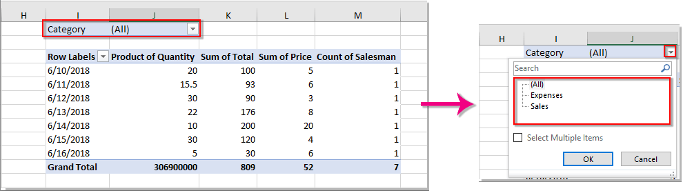
Consider the following example: The Pivot Table has a filter field named Category, with two filter values: “Expenses” and “Sales”. By linking a cell to the Pivot Table filter, you can control the displayed data by typing either “Expenses” or “Sales” in your chosen cell.
To implement this:
- Select the cell you want to use as the filter controller (e.g., cell H6), and enter one of your filter values in advance. Ensure the value exactly matches those available in the Pivot Table filter field.
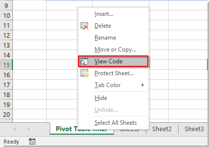
- Go to the worksheet containing your Pivot Table. Right-click on the sheet tab and choose View Code from the menu. This opens the Visual Basic for Applications window.
In the Microsoft Visual Basic for Applications window, paste the following VBA code into the code pane.
VBA code: Link Pivot Table filter to a certain cell
Private Sub Worksheet_Change(ByVal Target As Range)
'Update by Extendoffice 20180702
    Dim xPTable As PivotTable
    Dim xPFile As PivotField
    Dim xStr As String
    On Error Resume Next
    If Intersect(Target, Range("H6")) Is Nothing Then Exit Sub
    Application.ScreenUpdating = False
    Set xPTable = Worksheets("Sheet1").PivotTables("PivotTable2")
    Set xPFile = xPTable.PivotFields("Category")
    xStr = Target.Text
    xPFile.ClearAllFilters
    xPFile.CurrentPage = xStr
    Application.ScreenUpdating = True
End Sub
Notes:
After pasting the code, press Alt + Q to close the VBA editor window and return to Excel.
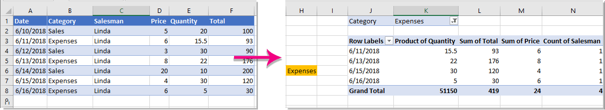
Now, the filter state of your Pivot Table is controlled by the content of cell H6. Simply changing the value in cell H6 (to "Sales" or "Expenses") will instantly update the Pivot Table's display. If you encounter any issues, please double-check that the referenced cell value exactly matches a filter value in the Pivot Table, and that names in your code are correctly assigned.
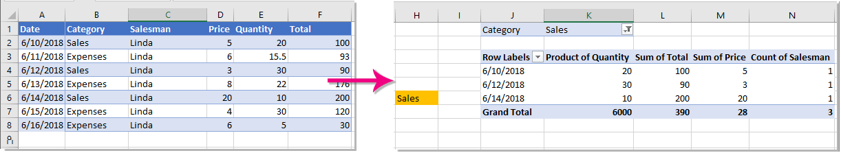
Whenever you modify the cell’s content, the Pivot Table refreshes its filtered data accordingly.
Tips and troubleshooting: If the filter field value in the cell does not match the available items exactly (including capitalization and spacing), the code may not apply the filter as expected. Always verify that your field and table names are spelled correctly in the VBA code. If you want to use this setup across multiple Pivot Tables, you can further adapt the code or extend it using Loops.

Unlock Excel Magic with Kutools AI
- Smart Execution: Perform cell operations, analyze data, and create charts—all driven by simple commands.
- Custom Formulas: Generate tailored formulas to streamline your workflows.
- VBA Coding: Write and implement VBA code effortlessly.
- Formula Interpretation: Understand complex formulas with ease.
- Text Translation: Break language barriers within your spreadsheets.
Excel Formula - Use formulas (e.g., GETPIVOTDATA) in conjunction with slicer or Report Filter referencing
Although Excel does not offer a purely native formulaic method to bind a Pivot Table’s filter directly to a cell, you can achieve dynamic reporting and display relevant values with formulas such as GETPIVOTDATA in combination with slicers or report filters. This solution is useful when you want to build dashboards where summary values update instantly based on a filter selection or another cell’s input, making data analysis more interactive.
Applicable scenarios include dynamic report panels, dashboards, or comparative summaries where you want the displayed result to follow slicer selections, or reflect data related to a cell’s contents. The main advantage is that this method works well for displaying updated summary data. However, the actual filter state of the pivot table cannot be programmatically set by cell formula alone.
Example: Displaying Pivot Table summary based on a cell value
Suppose you have a Pivot Table summarizing sales by Category (e.g., “Sales”, “Expenses”). You can use GETPIVOTDATA to extract the relevant value for a category specified in a cell.
1. Assume cell H6 contains the category you wish to display (e.g., “Sales”). Place the following formula in your summary cell (e.g., I6):
=GETPIVOTDATA("Sum of Amount",$B$4,"Category",H6)2. After entering the formula in I6, press Enter. Now, whenever you change H6 to a valid category (like "Expenses" or "Sales"), I6 will instantly update to show the total for that category, according to the current Pivot Table.
- The first argument “Sum of Amount” should be replaced with the actual name of the Values field in your Pivot Table (for example, "Total Sales" or whatever label your values use). Similarly, $B$4 should be replaced with the reference to any specific cell inside your Pivot Table—Excel will automatically recognize this reference and associate it with the correct Pivot Table for the GETPIVOTDATA function to work properly.
- To get your precise GETPIVOTDATA syntax, click into a cell of your Pivot Table and try to reference a value—Excel auto-generates the correct syntax. Make sure H6 matches one of the available categories in the table for accurate results.
Tip: While this method doesn’t change the filter within the Pivot Table itself, it effectively displays outcome data as though filtered by the cell, providing a dynamic display linked to your target cell input. You can also use this method to power charts, summary tables, or dashboards.
Troubleshooting: If the formula returns a #REF! or #VALUE! error, check that your cell references are correct, the entered category exists in your Pivot Table, and the field/sum name matches exactly.
Other Built-in Excel Methods - Connect Pivot Table Slicers and dashboards for interactive filtering
Excel’s Slicer and Report Filter tools provide user-friendly, built-in options for interactive filtering without writing VBA code. You can use these methods to achieve a dashboard-like effect, connecting multiple Pivot Tables or displays to one or more slicers.
One common approach is to insert a Slicer linked to your Pivot Table field (e.g., “Category”). Users simply click desired items in the slicer and the Pivot Table(s) update accordingly. If you have multiple Pivot Tables based on the same data source, you can connect a single slicer to all tables for synchronized filtering, making your reporting interface more intuitive and consistent.
To create a slicer and link it:
- Click into your Pivot Table and go to PivotTable Analyze (or Options tab, depending on Excel version) > Insert Slicer.
- Check the desired field (e.g., Category) and click OK. The slicer appears on the sheet and allows users to filter visually.
- To link one slicer to multiple Pivot Tables, right-click the slicer, choose Report Connections (or Pivottable Connections), and check all Pivot Tables you wish to synchronize.
This is especially powerful for dashboard scenarios where various visualizations respond together to user filters.
Advantages: Very easy to use for most interactive filtering needs and does not require macros or custom code. Great for dashboards or shared reports where simplicity and reliability are crucial. The limitation is that absolute cell-to-filter automation (cell-to-filter binding) is not natively supported—direct value-to-filter assignment needs VBA or external tools.
Troubleshooting: If a slicer doesn’t connect to multiple Pivot Tables, ensure all tables are built from the same cache/data source. The Report Connections option only appears if tables are compatible.
Summary suggestion: When choosing the optimal method for linking Pivot Table filters to cell values or building interactive dashboards, consider your required level of automation, Excel version limits, and whether VBA/macros are permitted in your environment. For basic needs, slicers and formulas (GETPIVOTDATA) provide quick, robust results. For advanced automation, the VBA solution delivers greater control. Always verify that field names and filter items are used consistently for accurate outcomes. If errors arise, check cell input values and ensure all names match exactly between code, formulas, and the data set.
Related articles:
- How to combine multiple sheets into a pivot table in Excel?
- How to create a Pivot Table from Text file in Excel?
- How to filter Pivot table based on a specific cell value in Excel?
Best Office Productivity Tools
Supercharge Your Excel Skills with Kutools for Excel, and Experience Efficiency Like Never Before. Kutools for Excel Offers Over 300 Advanced Features to Boost Productivity and Save Time. Click Here to Get The Feature You Need The Most...
Office Tab Brings Tabbed interface to Office, and Make Your Work Much Easier
- Enable tabbed editing and reading in Word, Excel, PowerPoint, Publisher, Access, Visio and Project.
- Open and create multiple documents in new tabs of the same window, rather than in new windows.
- Increases your productivity by 50%, and reduces hundreds of mouse clicks for you every day!
All Kutools add-ins. One installer
Kutools for Office suite bundles add-ins for Excel, Word, Outlook & PowerPoint plus Office Tab Pro, which is ideal for teams working across Office apps.
- All-in-one suite — Excel, Word, Outlook & PowerPoint add-ins + Office Tab Pro
- One installer, one license — set up in minutes (MSI-ready)
- Works better together — streamlined productivity across Office apps
- 30-day full-featured trial — no registration, no credit card
- Best value — save vs buying individual add-in