How to quickly find and remove all rows with errors in Excel?
Managing error values in Excel can be a frequent task, especially when errors disrupt your data analysis or calculations. Error values such as #DIV/0!, #N/A, #VALUE! can occur for various reasons—such as referencing invalid data, incorrect formulas, or importing data from external systems. Efficiently finding and removing all rows or cells that contain these errors is important for keeping your spreadsheets clean and reliable. This tutorial offers a comprehensive introduction to several practical methods for identifying and clearing error-filled cells and rows, using both built-in Excel features, formulas, VBA code, and specialized tools.
- Find and remove all cells with errors by Go To Special
- Find and remove all cells with errors by an advanced tool
- Remove all rows with errors with VBA
- Find and remove all rows with errors by an advanced filter tool
- Remove error rows using Excel formulas (helper columns)
- Highlight errors using Conditional Formatting
- Other relatived articles (operations) about filtering
Excel's Go To Special function allows you to quickly select all cells containing formula errors within a chosen range or on an entire worksheet. This method is best for sheets where you need to clear cell content regardless of which row they're in.
1. Select your target range or the whole worksheet as needed, then press Ctrl + G to open the Go To dialog box.
2. Click Special to launch the Go To Special dialog. Here, check the Formulas option, and within Formula options, ensure only the Errors checkbox is marked. This makes sure only error cells are selected.
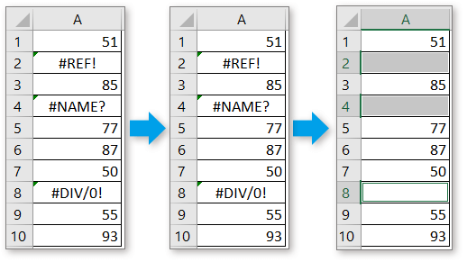
3. Click OK, and Excel will select every cell with a formula error in your range. You can then press the Delete key to clear their contents. 
Note: This only removes cell values, not entire rows, which is useful if you want to preserve other data in the row.
Applicable scenario: Quickly cleaning up formula errors in specific columns (not always suitable if you need to remove entire error-containing rows).
For a more streamlined and user-friendly approach, you can use the Select Cells with Error Value tool in Kutools for Excel. This feature allows you to immediately select all error values within your chosen range, making removal straightforward—especially when dealing with large or complex sheets.
1. Choose the range you wish to scan for errors, then click Kutools > Select > Select Cells with Error Value.
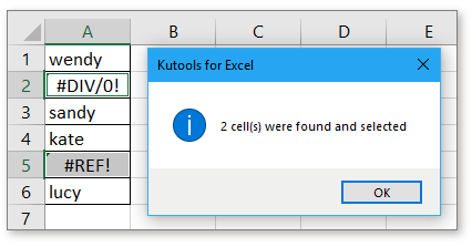
2. All error cells will be highlighted instantly. Click OK to close the reminder dialog, and press Delete to clear the error cells’ values.

In cases where you need to delete every row containing at least one error cell, a VBA macro is a flexible and powerful solution. This approach is recommended for large datasets or repetitive tasks, allowing you to automate error row removal and reduce manual effort.
1. Press Alt + F11 to open the Microsoft Visual Basic for Applications editor. In the window, select Insert > Module to open a blank code module.
2. Copy and paste the following VBA code into the module window:
VBA: Remove error rows
Sub DeleteErrorRows()
Dim xWs As Worksheet
Dim xRg As Range
Dim xFNum As Integer

   Set xWs = Application.ActiveSheet
Application.ScreenUpdating = False
    On Error Resume Next
    With xWs
        Set xRg = .UsedRange
        xRg.Select
        For xFNum = 1 To xRg.Columns.count
            With .Columns(xFNum).SpecialCells(xlCellTypeFormulas, xlErrors)
                .EntireRow.Delete
            End With
        Next xFNum
    End With
Application.ScreenUpdating = True
End Sub
3. Press F5 to run the code. All rows containing error values will be deleted automatically.
The Super Filter utility within Kutools for Excel streamlines filtering and removing rows with errors. This method is suitable when you need to apply specific error types or combine multiple criteria while filtering your data—especially helpful in complex tables with various error types.
After free installing Kutools for Excel (30-day free trial), follow these steps:
1. Highlight your target data range, then go to Kutools Plus > Super Filter to open the filter pane.
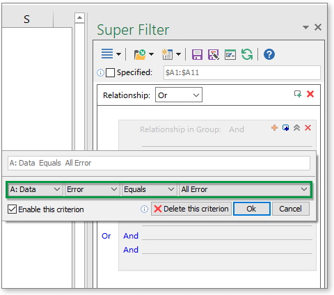
2. In the Super Filter pane, set the filtering criterion:
a) Choose the column header for error checking.
b) Select Error from the secondary drop-down menu.
c) Select Equals from the comparison drop-down.
d) Choose All Error in the final drop-down.
3. Click Ok to apply your criterion, then click Filter. The tool will display only those rows containing error values.
Error rows will now be isolated.
4. To remove these rows, select them individually, right-click, and choose Delete Row in the context menu.
Once deleted, click the Clear button in Super Filter to return to your full dataset.
Tip: You can use specific error types like #NAME? or #DIV/0! by customizing the filter settings.
Super Filter also supports multifaceted criteria that are not found in native Excel filters. Click for details.
Using Excel formulas in a helper column is a practical solution for detecting rows containing error values, especially if you want to decide which errors should prompt row removal. This method provides transparency and flexibility, making it easy to audit which rows are flagged and manually or automatically filter and delete them.
Applicable scenario: When you want granular control over which errors are flagged, or to keep audit information before deletion. This is ideal for tables where errors may be spread across multiple columns.
1. Add a new helper column at the rightmost edge (e.g., column D) and enter the following formula in cell D2 to check for errors across column B:
=ISERROR(B2)Replace B2 with the cell reference where errors may occur. For other error types, you can use:
=ISERR(B2) (Detects any error except #N/A)
=ISNA(B2) (Detects #N/A errors only)
=IFERROR(B2,"Error") (Returns custom label for errors)
2. Drag the formula down to fill the helper column for all rows in your dataset. Each cell will show TRUE if an error exists, FALSE if not.
3. Use Excel's filter: Click the filter drop-down in your helper column and filter to show rows where the formula is TRUE. Delete these rows as needed, then remove the helper column once finished.
Practical tip: You can expand the formulas to scan multiple columns (e.g., =OR(ISERROR(B2),ISERROR(C2))) and flag rows where any cell has an error. If you use IFERROR, you can also display a custom message beside errors for easier review before removal.
Caution: If your data includes intentional errors for other analysis reasons, review flagged rows before deleting.
Conditional Formatting in Excel enables you to automatically highlight cells or rows that contain error values, making them easy to spot for review or deletion. This method is useful when you need visual cues before deciding which data to keep or remove, and it can complement other approaches for enhanced accuracy.
Scenario: Ideal for quality control in large datasets where visual inspection is needed, or before sharing data with others.
- Select the range where you want to highlight errors.
- Go to Home > Conditional Formatting > New Rule > Use a formula to determine which cells to format.
- Enter this formula to target errors (e.g. for column B):
Adjust reference as necessary for your sheet.=ISERROR(B2) - Click Format, choose a highlight color, then click OK to apply.
- All error cells will be highlighted; you can now manually review and remove entire rows as desired.
Practical tip: Always review highlighted cells before deleting rows, especially if some errors are expected or temporarily present during data entry.
Summing up and troubleshooting: When working with error values in Excel, always choose a method suited to your dataset's size, complexity, and whether you intend to remove cells or entire rows. Use helper columns and the filter function for customizable error detection, conditional formatting for visual cues, and advanced tools when handling large or irregular tables. Before executing mass deletions, back up your file! If unexpected errors occur (e.g., formulas not detecting errors, rows not deleting), double-check cell references and ensure all relevant columns are included in your criteria. Kutools solutions offer extended functionality for tricky scenarios, but even built-in Excel features can help keep your sheets tidy and professional.
Filter data based on a list
This tutorial provides tricks on filtering data based on a given list data in Excel.
Filter data contains asterisk
As we know, we use asterisk mask to stand any characters when you filter data, but how can you do if you want to filter data which contains asterisk mask? Now this article introduces the method about data filtering if containing asterisk or other special characters in Excel.
Filter data with criteria or wildcard
If you want to filter data with multiple criteria, how can you do? This tutorial is talking about how to set multiple criteria and filter data in Excel.
Best Office Productivity Tools
Supercharge Your Excel Skills with Kutools for Excel, and Experience Efficiency Like Never Before. Kutools for Excel Offers Over 300 Advanced Features to Boost Productivity and Save Time. Click Here to Get The Feature You Need The Most...
Office Tab Brings Tabbed interface to Office, and Make Your Work Much Easier
- Enable tabbed editing and reading in Word, Excel, PowerPoint, Publisher, Access, Visio and Project.
- Open and create multiple documents in new tabs of the same window, rather than in new windows.
- Increases your productivity by 50%, and reduces hundreds of mouse clicks for you every day!
All Kutools add-ins. One installer
Kutools for Office suite bundles add-ins for Excel, Word, Outlook & PowerPoint plus Office Tab Pro, which is ideal for teams working across Office apps.
- All-in-one suite — Excel, Word, Outlook & PowerPoint add-ins + Office Tab Pro
- One installer, one license — set up in minutes (MSI-ready)
- Works better together — streamlined productivity across Office apps
- 30-day full-featured trial — no registration, no credit card
- Best value — save vs buying individual add-in