Return multiple matching values based on multiple criteria in Excel (Full guide)
Excel users frequently encounter scenarios where it is necessary to extract multiple values that satisfy several criteria simultaneously, and present all matching results in a column, a row, or consolidated within a single cell. This guide explores methods for all Excel versions as well as the newer FILTER function available in Excel 365 and 2021.
Return multiple matching values based on multiple criteria in a single cell
In Excel, extracting multiple matching values based on multiple criteria within a single cell is a common challenge. Here explore two efficient methods.
Method 1: Using the Textjoin function (Excel365 / 2021,2019)
To get all matching values into a single cell with delimiters, the TEXTJOIN function can do you a favor.
Enter or copy the following formula into a blank cell, then press Enter key (Excel 2021 and Excel 365) or Ctr l+ Shift + Enter keys in Excel 2019 to get the result:
=TEXTJOIN(", ", TRUE, IF(($A$2:$A$18=E2)*($B$2:$B$18=F2), $C$2:$C$18, ""))
- ($A$2:$A$21=E2)*($B$2:$B$21=F2) check whether each row meets both conditions: “Seller equals E2” and “Month equals F2.” If both conditions are met, the result is 1; otherwise, it is 0. The asterisk * means both conditions must be true.
- IF(..., $C$2:$C$21, "") returns the product name if the row matches; otherwise, it returns a blank.
- TEXTJOIN(", ", TRUE, ...) combines all the non-blank product names into one cell, separated by ", ".
Method 2: Using Kutools for Excel
Kutools for Excel offers a powerful yet simple solution, allowing you to quickly retrieve and combine multiple matches into a single cell based on multiple criteria without complex formulas.
After installing Kutools for Excel, please do as this:
- Select the data range that you want to get all corresponding values based on criteria.
- Then, click Kutools > Merge & Split > Advanced Combine Rows, see screenshot:

- In the Advanced Combine Rows dialog box, please configure the following options:
- Choose the column headers that contain your matching criteria (e.g., Seller and Month). For each selected column, click Primary Key to define them as your lookup conditions.
- Click the column header where you want the combined results (e.g., Product). From the Combine section, select your preferred delimiter (e.g., comma, space, or custom separator).
- At last, click OK button.


Result: Kutools will instantly merge all matching values into a single cell per unique criteria combination.
Return multiple matching values based on multiple criteria in a column
When you need to extract and display multiple matching records from a dataset based on several conditions, returning the results in a vertical column format, Excel offers several powerful solutions.
Method 1: Using an array formula (for all versions)
You can use the following array formula to return results vertically in a column:
1. Copy or enter the following formula into a blank cell:
=IFERROR(INDEX($C$2:$C$18, SMALL(IF(($A$2:$A$18=$E$2)*($B$2:$B$18=$F$2), ROW($C$2:$C$18)-ROW($C$2)+1), ROW(1:1))), "")2. Press Ctrl + Shift + Enter keys to get the first matching result, and then select the first formula cell and drag the fill handle down to the cells until blank cell is displayed, now, all matching values are returned as below screenshot shown:

- $A$2:$A$18=$E$2: Checks if the Seller matches the value in cell E2.
- $B$2:$B$18=$F$2: Checks if the Month matches the value in cell F2.
- * is a logical AND operator (both conditions must be true).
- ROW($C$2:$C$18)-ROW($C$2)+1: Generates a relative row number for each product.
- SMALL(..., ROW(1:1)): Fetches the n-th smallest matching row (as the formula is dragged down).
- INDEX(...): Returns the product from the matching row.
- IFERROR(..., ""): Returns a blank cell if there are no more matches.
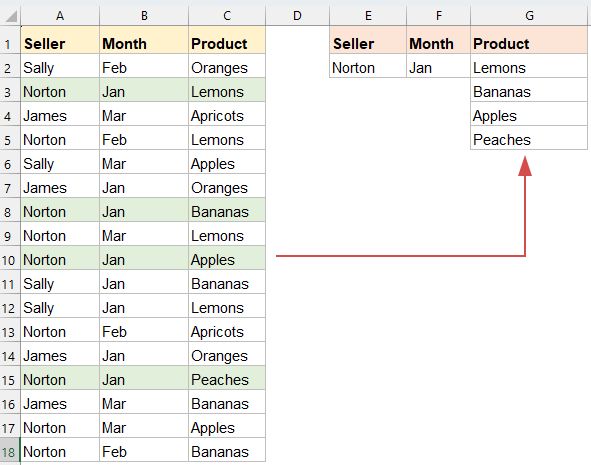
Method 2: Using Filter function (Excel365 / 2021)
If you are using Excel 365 or Excel 2021, the FILTER function is an excellent choice for returning multiple results based on multiple criteria, thanks to its simplicity, clarity, and ability to dynamically spill results without complex array formulas.
Copy or enter the below formula into a blank cell, then press Enter key, all matching records are returned based on the multiple criteria.
=FILTER(C2:C18, (A2:A18=E2)*(B2:B18=F2), "No match")
- FILTER(...) returns all values from C2:C18 where both conditions are met.
- (A2:A18=E2)*(B2:B18=F2): Logical array that checks for matching seller and month.
- "No match": Optional message if no values are found.
Return multiple matching values based on multiple criteria in a row
Excel users often need to extract multiple values from a dataset that meet several conditions and display them horizontally (in a row). This is useful for creating dynamic reports, dashboards, or summary tables where vertical space is limited. In this section, we’ll explore two powerful methods.
Method 1: Using an array formula (for all versions)
Traditional array formulas allow extracting multiple matching values using INDEX, SMALL, IF, and COLUMN functions. Unlike vertical extraction (column-based), we adjust the formula to return results in a row.
1. Copy or enter the below formula into a blank cell:
=IFERROR(INDEX($C$2:$C$18, SMALL(IF(($A$2:$A$18=$E$2)*($B$2:$B$18=$F$2), ROW($C$2:$C$18)-ROW($C$2)+1), COLUMN(A1))), "")2. Press Ctrl + Shift + Enter keys to get the first matching result, and then select the first formula cell and drag the formula to the right across columns to retrieve all results.

- $A$2:$A$18=$E$2: Checks if the Seller matches.
- $B$2:$B$18=$F$2: Checks if the Month matches.
- *: Logical AND—both conditions must be true.
- ROW($C$2:$C$18)-ROW($C$2)+1: Creates relative row numbers.
- COLUMN(A1): Adjusts which match to return, depending on how far the formula has been dragged right.
- IFERROR(...): Prevents errors once matches are exhausted.
Method 2: Using Filter function (Excel365 / 2021)
Copy or enter the below formula into a blank cell, then press Enter key, all matching values are extracted and located in a row. See screenshot:
=TRANSPOSE(FILTER(C2:C18, (A2:A18=E2)*(B2:B18=F2), "No match"))
- FILTER(...): Retrieves matching values from column C based on the two conditions.
- (A2:A18=E2)*(B2:B18=F2): Both conditions must be true.
- TRANSPOSE(...): Converts the vertical array returned by FILTER into a horizontal array.
🔚 Conclusion
Retrieving multiple matching values based on multiple criteria in Excel can be accomplished in several ways, depending on how you want to display the results—whether in a column, a row, or within a single cell.
- For users with Excel 365 or Excel 2021, the FILTER function offers a modern, dynamic, and elegant solution that minimizes complexity.
- For those using older versions, array formulas remain powerful tools, though they require a bit more setup and care.
- Additionally, if you want to consolidate results into a single cell or prefer a no-code solution, the TEXTJOIN function or third-party tools like Kutools for Excel can significantly streamline the process.
Choose the method that best fits your version of Excel and your preferred layout, and you’ll be well-equipped to handle multi-criteria lookups efficiently and accurately. If you're interested in exploring more Excel tips and tricks, our website offers thousands of tutorials to help you master Excel.
More relative articles:
- Return Multiple Lookup Values In One Comma Separated Cell
- In Excel, we can apply the VLOOKUP function to return the first matched value from a table cells, but, sometimes, we need to extract all matching values and then separated by a specific delimiter, such as comma, dash, etc… into a single cell as following screenshot shown. How could we get and return multiple lookup values in one comma separated cell in Excel?
- Vlookup And Return Multiple Matching Values At Once In Google Sheet
- The normal Vlookup function in Google sheet can help you to find and return the first matching value based on a given data. But, sometimes, you may need to vlookup and return all matching values as following screenshot shown. Do you have any good and easy ways to solve this task in Google sheet?
- Vlookup And Return Multiple Values From Drop Down List
- In Excel, how could you vlookup and return multiple corresponding values from a drop down list, which means when you choose one item from the drop down list, all of its relative values are displayed at once as following screenshot shown. This article, I will introduce the solution step by step.
- Vlookup And Return Multiple Values Vertically In Excel
- Normally, you can use the Vlookup function to get the first corresponding value, but, sometimes, you want to return all matching records based on a specific criterion. This article, I will talk about how to vlookup and return all matching values vertically, horizontally or into one single cell.
- Vlookup And Return Matching Data Between Two Values In Excel
- In Excel, we can apply the normal Vlookup function to get the corresponding value based on a given data. But, sometimes, we want to vlookup and return the matching value between two values as the following screenshot shown, how could you deal with this task in Excel?
Best Office Productivity Tools
Supercharge Your Excel Skills with Kutools for Excel, and Experience Efficiency Like Never Before. Kutools for Excel Offers Over 300 Advanced Features to Boost Productivity and Save Time. Click Here to Get The Feature You Need The Most...
Office Tab Brings Tabbed interface to Office, and Make Your Work Much Easier
- Enable tabbed editing and reading in Word, Excel, PowerPoint, Publisher, Access, Visio and Project.
- Open and create multiple documents in new tabs of the same window, rather than in new windows.
- Increases your productivity by 50%, and reduces hundreds of mouse clicks for you every day!
All Kutools add-ins. One installer
Kutools for Office suite bundles add-ins for Excel, Word, Outlook & PowerPoint plus Office Tab Pro, which is ideal for teams working across Office apps.
- All-in-one suite — Excel, Word, Outlook & PowerPoint add-ins + Office Tab Pro
- One installer, one license — set up in minutes (MSI-ready)
- Works better together — streamlined productivity across Office apps
- 30-day full-featured trial — no registration, no credit card
- Best value — save vs buying individual add-in