20+ VLOOKUP Examples For Excel Beginner & Advanced Users
The VLOOKUP function is one of the most popular functions in Excel. This tutorial will introduce how to use VLOOKUP function in Excel with dozens of basic and advanced examples step by step.
Download VLOOKUP sample files
Basic Vlookup examples | Advanced Vlookup examples | Vlookup keep cell formatting
Introduction of VLOOKUP function – Syntax and Arguments
In Excel, the VLOOKUP function is a powerful function for most of Excel users, it allows you to look for a value in the leftmost of the data range, and return a matching value in the same row from a column you specified as following screenshot shown.
The syntax of VLOOKUP function:
Arguments:
"Lookup_value" (required): The value that you want to search. It can be a value (number, date or text) or cell reference. It must be in the first column of the table_array range.
"Table_array" (required): The data range or table where the lookup value column and the result value column are located.
"Col_index_num" (required): The column number that contains the return values. It starts with 1 from the leftmost column in the table array.
"Range_lookup" (optional): A logical value that determines whether this VLOOKUP function will return an exact match or an approximate match.
- "Approximate match" – 1 / TRUE / omitted (default): If an exact match is not found, the formula searches for the closest match - the largest value that is smaller than the lookup value.
- "Exact match" – 0 / FALSE: This is used to search for a value exactly equal to the lookup value. If an exact match is not found, the error value #N/A will be returned.
Function Notes:
- The Vlookup function only looks for a value from left to right.
- The Vlookup function performs a case-insensitive lookup.
- If there are multiple matching values based on the look up value, only the first matched will be returned by using the Vlookup function.
Basic VLOOKUP examples
In this section, we will talk about some Vlookup formulas you used frequently.
2.1.1 Do an exact match VLOOKUP
Normally, if you are looking for an exact match with the VLOOKUP function, you just need to use FALSE as the last argument.
For example, to get the corresponding Math scores based on the specific ID numbers, please do as this:
Please copy and paste the below formula into a blank cell (here, I select G2), and press "Enter" key to get the result:
=VLOOKUP(F2,$A$2:$D$7,3,FALSE)
Note: In the above formula, there are four arguments:
- "F2" is the cell that contains the value C1005 you want to lookup;
- "A2:D7" is the table array in which you are performing the lookup;
- "3" is the column number that your matched value is returned from; (Once the function spots the ID - C1005, it will go to the third column of the table array, and return the values in the same row as that of the ID - C1005. )
- "FALSE" refers to the exact match.
How the VLOOKUP formula works?
First, it looks for the ID - C1005 in the left-most column of the table. It goes from top to bottom and finds the value in cell A6.
As soon as it finds the value, it will turn right to the third column and extracts the value in it. 
So, you will get the result as below screenshot shown:
Kutools for Excel Boasts Over 300 Features, Ensuring That What You Need is Just A Click Away...
2.1.2 Do an approximate match VLOOKUP
The approximate match is useful for searching values between data ranges. If the exact match is not found, the approximate VLOOKUP will return the largest value that is smaller than the lookup value.
For example, if you have the following range of data, and the specified orders are not in the Orders column, how to get its closest Discount in column B? 
Step 1: Apply the VLOOKUP formula and fill it to other cells
Copy and paste the following formula into a cell where you want to put the result, and then drag the fill handle down to apply this formula to other cells.
=VLOOKUP(D2,$A$2:$B$9,2,TRUE)Result:
Now, you will get the approximate matches based on the given values, see screenshot:
Notes:
- In the above formula:
- "D2" is the value that you want to return its relative information;
- "A2:B9" is the data range;
- "2" indicates the column number that your matched value is returned;
- "TRUE" refers to the approximate match.
- The approximate match will return the largest value that is smaller than your specific lookup value if no exact match is found.
- To use the VLOOKUP function to get an approximate match value, you must sort the leftmost column of the data range in ascending order, otherwise it will return a wrong result.
2.2 Do a case sensitive VLOOKUP in Excel
By default, the VLOOKUP function performs a case insensitive lookup which means it treats lowercase and uppercase characters as identical. Sometime, you may need to perform a case-sensitive lookup in Excel, the normal VLOOKUP function may not solve it. In this case, you can use alternative functions such as INDEX and MATCH with the EXACT function, or the LOOKUP and EXACT functions.
For example, I have the following data range which ID column contains text string with upper case or lower case, now, I want to return the corresponding Math score of the given ID number.
Step 1: Apply any one formula and fill it to other cells
Please copy and paste any one of the below formulas into a blank cell where you want to get the result. Then,select the formula cell, drag the fill handle down to the cells where you want to fill this formula.
Formula 1: After pasting the formula, please press "Ctrl" + "Shift" + "Enter" keys.
=INDEX($C$2:$C$10,MATCH(TRUE,EXACT(F2,$A$2:$A$10),0))Formula 2: After pasting the formula, please press "Enter" key.
=LOOKUP(2,1/EXACT(F2,$A$2:$A$10),$C$2:$C$10)Result:
Then you will get the correct results you need. See screenshot:
Notes:
- In the above formula:
- "A2:A10" is the column which contains the specific values you want to look up in;
- "F2" is the lookup value;
- "C2:C10" is the column where the result will be returned from.
- If multiple matches are found, this formula will always return the last match.
2.3 VLOOKUP values from right to left in Excel
The VLOOKUP function always searches a value in the leftmost column of a data range and returns the corresponding value from a column to the right. If you want to perform a reverse VLOOKUP which means to lookup a specific value in the right column and return its corresponding value in left column as below screenshot shown:
Click to know the details step by step about this task…

2.4 VLOOKUP the second, nth or last matching value in Excel
Normally, if multiple matching values are found when using the Vlookup function, only the first matched record will be returned. In this section, I will talk about how to get the second, nth or last matching value in a data range.
2.4.1 VLOOKUP and return the 2nd or nth matching value
Suppose you have a list of names in column A, the training course they purchased in column B. Now, you are looking to find the 2nd or nth training course bought by the given customer. See screenshot:
Here, the VLOOKUP function may not solve this task directly. But, you can use the INDEX function as an alternative.
Step 1: Apply and fill the formula to other cells
For instance, to get the second matching value based on the given criteria, please apply the following formula into a blank cell, and press "Ctrl" + "Shift" + "Enter" keys together to get the first result. And then, select the formula cell, drag the fill handle down to the cells where you want to fill this formula.
=INDEX($B$2:$B$14,SMALL(IF(E2=$A$2:$A$14,ROW($A$2:$A$14)-ROW($A$2)+1),2))Result:
Now, all the second matched values based on the given names have been displayed at once.
Note: In the above formula:
- "A2:A14" is the range with all the values for lookup;
- "B2:B14" is the range of the matching values you want to return from;
- "E2" is the lookup value;
- "2" indicates the second matched value you want to get, to return the third matching value, you just need to change it to 3.
2.4.2 VLOOKUP and return the last matching value
If you want to vlookup and return the last matching value as below screenshot shown, this VLOOKUP And Return The Last Matching Value tutorial may help you to get the last matching value in details.

2.5 VLOOKUP matching values between two given values or dates
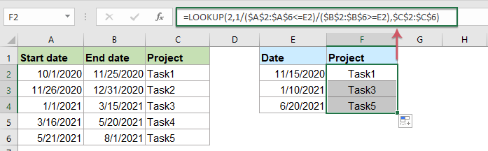
Sometimes, you may want to lookup values between two values or dates and return the corresponding results as shown in the screenshot below. In such case, you can use the LOOKUP function instead of VLOOKUP function with a sorted table.
2.5.1 VLOOKUP matching values between two given values or dates with formula
Step 1: Arrange the data and apply the following formula
Your original table should be a sorted data range. And then, copy or enter the following formula into a blank cell.Then, drag the fill handle to fill this formula to other cells you need.
=LOOKUP(2,1/($A$2:$A$6<=E2)/($B$2:$B$6>=E2),$C$2:$C$6)Result:
And now, you will get all matched records based on the given value, see screenshot:
Notes:
- In the above formula:
- "A2:A6" is the range of smaller values;
- "B2:B6" is the range of larger numbers;
- "E2" is the lookup value which you want to get its corresponding value;
- "C2:C6" is the column from which you want to return a corresponding value.
- This formula also can be used for extracting matched values between two dates as below screenshot shown:

2.5.2 VLOOKUP matching values between two given values or dates with a handy feature
If you find it difficult to remember and understand the above formula, here, I will introduce an easy tool – "Kutools for Excel", with its "LOOKUP between Two Values feature", you can return the corresponding item based on the specific value or date between two values or dates with ease.
- Click "Kutools" > "Super LOOKUP" > "LOOKUP between Two Values" to enable this feature.
- Then specify the operations from the dialog box based on your data.

2.6 Using wildcards for partial matches in VLOOKUP function
In Excel, the wildcards can be used within the VLOOKUP function, which allows you to perform a partial match on a lookup value. For instance, you can use VLOOKUP to return matched value from a table based on part of a lookup value.
Supposing, I have a range of data as below screenshot shown, now, I want to extract the score based on the first name (not full name). How could solve this task in Excel?
Step 1: Apply the formula and fill to other cells
Please copy or enter the following formula into a blank cell, and then, drag the fill handle to fill this formula to other cells you need:
=VLOOKUP(E2&"*", $A$2:$C$11, 3, FALSE)Result:
And all the matched scores have been returned as below screenshot shown:
Note: In the above formula:
- "E2&”*”" is the criteria for the partial math. This means you are looking for any value that starts with the value in cell E2. (The wildcard “*” indicates any one character or any characters)
- "A2:C11" is the range of data where you want to search for the matched value;
- "3" means to return the matching value from the 3rd column of the data range;
- "False" indicates the exact math. ( When using wildcards, you must set the last argument in the function as FALSE or 0 to enable exact match mode in VLOOKUP function.)
- To find and return the matching values ending with a specific value, you should put the wildcard "*" in front of the value. Please apply this formula:
-
=VLOOKUP("*"&E2, $A$2:$C$11, 3, FALSE)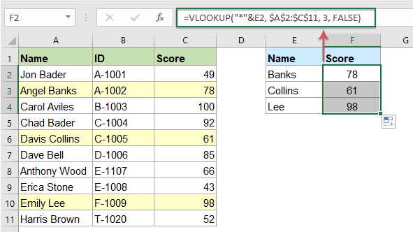
- To lookup and return the matched value based on part of the text string, whether the specified text is at the bebinning, end or in the middle of the text string, you just need to enclose the cell reference or text with two asterisks (*) on both sides. Please do with this formula
-
=VLOOKUP("*"&D2&"*", $A$2:$B$11, 2, FALSE)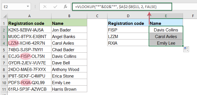


2.7 VLOOKUP values from another worksheet
Usually, you may have to work with more than one worksheet, the VLOOKUP function can be used to lookup data from another sheet as the same as on one worksheet.
For example, you have two worksheets as below screenshot shown, to lookup and return the corresponding data from the worksheet you specified, please do with the following steps:
Step 1: Apply the formula and fill to other cells
Please enter or copy the below formula into a blank cell where you want to get the matched items. Then, drag the fill handle down to the cells that you want to apply this formula.
=VLOOKUP(A2,'Data sheet'!$A$2:$C$15,3,0)Result:
You will get the corresponding results as you need, see screenshot:
 |  |
Note: In the above formula:
- "A2" represents the lookup value;
- "'Data sheet'!A2:C15" indicates to search the values from the range A2:C15 on the worksheet named Data sheet; (If the sheet name contains space or punctuation characters, you should enclose the sheet name in single quotes, otherwise, you can directly use the sheet name like:
=VLOOKUP(A2,Datasheet!$A$2:$C$15,3,0) ). - "3" is the column number which contains matched data you want to return from;
- "0" means to perform an exact match.
2.8 VLOOKUP values from another workbook
This section will talk about lookup and return the matching values from a different workbook by using the VLOOKUP function.
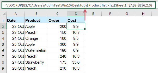
For example, let's say you have two workbooks. The first workbook contains a list of products and their respective costs. In the second workbook, you want to extract the corresponding cost for each product item as below screenshot shown.
Step 1: Apply the formula
Open both the workbooks you want to use, then apply the following formula into a cell where you want to put the result in the second workbook.Then, drag and copy this formula to other cells you need
=VLOOKUP(B2,'[Product list.xlsx]Sheet1'!$A$2:$B$6,2,0)Result:

Notes:
- In the above formula:
- "B2" represents the lookup value;
- "'[Product list.xlsx]Sheet1'!A2:B6" indicates to search from the range A2:B6 on the sheet named Sheet1 from the workbook Product list; (The reference to workbook is enclosed in square brackets, and the entire workbook + sheet is enclosed in single quotes.)
- "2" is the column number which contains matched data you want to return from;
- "0" indicates to return an exact match.
- If the lookup workbook is closed, the full file path for the lookup workbook will be shown in the formula as following screenshot shown:

2.9 Return blank or specific text instead of 0 or #N/A error
Usually, when you use the VLOOKUP function to return a corresponding value, if the matching cell is blank, it will return 0. And if the matching value is not found, you will get an error value of #N/A as shown in the screenshot below. If you want to display a blank cell or a specific value instead of 0 or #N/A, this VLOOKUP To Return Blank Or Specific Value Instead Of 0 Or N/A tutorial may do you a favor.

3.1 Two-way lookup (VLOOKUP in row and column)
Sometimes, you may need perform a 2-dimensional lookup, which means to search for a value in both row and column at the same time. For example, if you have the following data range, and you may need to get the value for a particular product in a specified quarter. This section will introduce a formula for dealing with this job in Excel.
In Excel, you can use a combination of VLOOKUP and MATCH functions to do a two-way lookup.
Please apply the following formula into a blank cell, and then press "Enter" key to get the result.
=VLOOKUP(G2, $A$2:$E$7, MATCH(H1, $A$2:$E$2, 0), FALSE)
Note: In the above formula:
- "G2" is the lookup value in the column that you want to get the corresponding value based on;
- "A2:E7" is the data table you will look from;
- "H1" is the lookup value in the row that you want to get the corresponding value based on;
- "A2:E2" is the cells of column headers;
- "FALSE" indicates to get an exact match.
3.2 VLOOKUP matching value based on two or more criteria
It is easy for you to look up the matching value based on one criterion, but if you have two or more criteria, what can you do?
3.2.1 VLOOKUP matching value based on two or more criteria with formulas
In this case, the LOOKUP or MATCH and INDEX functions in Excel can help you to solve this job quickly and easily.
For example, I have the below data table, to return the matched price based on the specific product and size, the following formulas may help you.
Step 1: Apply any of the formula below
Formula 1: Enter the following formula and press "Enter".
=LOOKUP(2,1/($A$2:$A$12=G1)/($B$2:$B$12=G2),($D$2:$D$12))Formula 2: Enter the following formula and press "Ctrl" + "Shift" + "Enter".
=INDEX($D$2:$D$12,MATCH(1,($A$2:$A$12=G1)*($B$2:$B$12=G2),0))Result:

Notes:
- In the above formulas:
- "A2:A12=G1" means to search the criteria of G1 in range A2:A12;
- "B2:B12=G2" means to search the criteria of G2 in range B2:B12;
- "D2:D12" is the range which you want to return the corresponding value from.
- If you have more than two criteria, you just need to join the other criteria into the formula, such as:
=LOOKUP(2,1/($A$2:$A$12=G1)/($B$2:$B$12=G2)/($C$2:$C$12=G3),($D$2:$D$12))=INDEX($D$2:$D$12,MATCH(1,($A$2:$A$12=G1)*($B$2:$B$12=G2)*($C$2:$C$12=G3),0)) 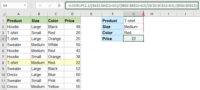

3.2.2 VLOOKUP matching value based on two or more criteria with Kutools for Excel
It can be challenging to remember the above complex formulas that need to be applied repeatedly, which can slow down your work efficiency. However, "Kutools for Excel" offers a "Multi-condition Lookup" feature that allows you to return the corresponding result based on one or more conditions with just only several clicks.
- Click "Kutools" > "Super LOOKUP" > "Multi-condition Lookup" to enable this feature.
- Then specify the operations from the dialog box based on your data.

3.3 VLOOKUP to return multiple values with one or more criteria
In Excel, the VLOOKUP function searches for a value and only return the first matching value if there are multiple corresponding values found. Sometimes, you may want to return all the corresponding values in a row, in a column or in a single cell. This section will talk about how to return the multiple matching values with one or more conditions in a workbook.
3.3.1 VLOOKUP all matching values based on one or more conditions horizontally
Assuming that you have a table of data that contain country, city and names in the range A1:C14, and now, you want to return all names horizontally which are from "US" as below screenshot shown. To solve this task, please click here to get the result step by step.

3.3.2 VLOOKUP all matching values based on one or more conditions vertically
If you need to Vlookup and return all matching values vertically based on specific criteria as below screenshot shown, please click here to get the solution in details.

3.3.3 VLOOKUP all matching values based on one or more conditions into single cell
If you want to Vlookup and return multiple matched values into a single cell with specified separator, the new function of TEXTJOIN can help you to solve this job quickly and easily.

Notes:
- The TEXTJOIN function is only available in Excel 2019, Excel 365 and later versions.
- If you use Excel 2016 and earlier versions, please use the User Defined Function of below article:
- Vlookup To Return Multiple Values In One Cell In Excel
3.4 VLOOKUP to return entire row of a matched cell
In this section, I will talk about how to retrieve the entire row of a matched value by using the VLOOKUP function.
Step 1: Apply the following formula
Please copy or type the below formula into a blank cell where you want to output the result, and press "Enter" key to get the first value. Then, drag the formula cell to the right until the data of the entire row is displayed.
=VLOOKUP($F$2,$A$1:$D$12,COLUMN(A1),FALSE)Result:
Now, you can see the entire row data is returned. See screenshot:
Note: in the above formula:
- "F2" is the lookup value you want to return the whole row based on;
- "A1:D12" is the data range you want to search for the lookup value from;
- "A1" indicates the first column number within your data range;
- "FALSE" indicates exact lookup.
Tips:
- If multiple rows are found based on the matched value, to return all of the corresponding rows, please apply the below formula, then press "Ctrl" + "Shift" + "Enter" keys together to get the first result. Then drag the fill handle to the right. And then, go on dragging the fill handle down across the cells to get all matching rows. See the demo below:
=IFERROR(INDEX(A:A,SMALL(IF(ISNUMBER(SEARCH($F$2,$A$2:$A$12)),ROW($A$2:$A$12),""),ROW()-1)),"")
3.5 Nested VLOOKUP in Excel
Sometimes, you may need to look up values which are interlinked across multiple tables. In this case, you can nest multiple VLOOKUP function together to get the final value.
For example, I have a worksheet that contains two separate tables. The first table lists all the product names along with their corresponding salesman. The second table lists the total sales of each salesman. Now, if you want to find the sales of each product, as shown in the following screenshot, you can nest the VLOOKUP function to accomplish this task. 
The generic formula for nested VLOOKUP function is:
Notes:
- "lookup_value" is the value you are looking for;
- "Table_array1", "Table_array2" are the tables in which the lookup value and return value exist;
- "col_index_num1" indicates the column number in the first table for finding the intermediate common data;
- "col_index_num2" indicates the column number in the second table that you want to return the matching value;
- "0" is used for an exact match.
Step 1: Apply and fill the following formula
Please apply the following formula into a blank cell, and then drag the fill handle down to the cells that you want to apply this formula.
=VLOOKUP(VLOOKUP(G3,$A$3:$B$7,2,0),$D$3:$E$7,2,0)Result:
Now, you will get the result as shown in the following screenshot:
Notes: in the above formula:
- "G3" contains the value you are looking for;
- "A3:B7", "D3:E7" are the table ranges in which the lookup value and return value exist;
- "2" is the column number in the range to return the matching value from.
- "0" indicates VLOOKUP exact math.
3.6 Check if value exists based on a list data in another column
The VLOOKUP function also can help you to check if values exist based on the data list in another column. For example, if you want to look for the names in column C and just return Yes or No if the name is found or not in column A as below screenshot shown.
Step 1: Apply the following formula
Please apply the following formula into a blank cell, then, drag the fill handle down to the cells that you want to fill this formula.
=IF(ISNA(VLOOKUP(C2,$A$2:$A$10,1,FALSE)), "No", "Yes")Result:
And you will get the result as you need, see screenshot:
Notes: in the above formula:
- "C2" is the lookup value you want to check;
- "A2:A10" is the list of range from where to check if the lookup values will be found or not;
- "FALSE" indicates to get an exact match.
3.7 VLOOKUP and sum all matched values in rows or columns
When working with numerical data, you may need to extract matched values from a table and sum the numbers in several columns or rows. This section will introduce some formulas that can help you accomplish this task.
3.7.1 VLOOKUP and sum all matched values in a row or multiple rows
Suppose you have a product list with sales for several months, as shown in the following screenshot. Now, you need to sum all orders in all months based on the given products.
Step 1: Apply the following formula
Please copy or enter the following formula into a blank cell, and then press "Ctrl" + "Shift" + "Enter" keys together to get the first result. Then, drag the fill handle down to copy this formula to other cells you need.
=SUM(VLOOKUP(H2, $A$2:$F$9, {2,3,4,5,6}, FALSE))
Result:
All the values in a row of the first matching value have been summed together, see screenshot:
Notes: in the above formula:
- "H2" is the cell containing the value you are looking for;
- "A2:F9" is the data range (without column headers) which include the lookup value and the matched values;
- "{2,3,4,5,6}" are column numbers used to calculate the total of the range;
- "FALSE" indicates an exact match.
Tip: If you want to sum all matches in multiple rows, please use the following formula:
-
=SUMPRODUCT(($A$2:$A$9=H2)*$B$2:$F$9) 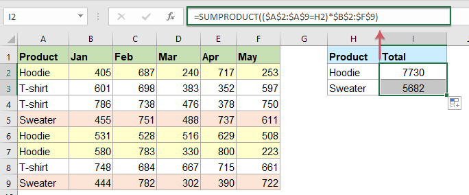

3.7.2 VLOOKUP and sum all matched values in a column or multiple columns
If you want to sum the total value for the specific months as shown in the screenshot below. The normal VLOOKUP function may not help you, here, you should apply the SUM, INDEX and MATCH functions together to create a formula.
Step 1: Apply the following formula
Apply the below formula into a blank cell, and then drag the fill handle down to copy this formula to other cells.
=SUM(INDEX($B$2:$F$9,0,MATCH(H2,$B$1:$F$1,0)))Result:
Now, the first matched values based on the specific month in a column have been summed together, see screenshot:
Notes: in the above formula:
- "H2" is the cell containing the value you are looking for;
- "B1:F1" is the column headers that contain the lookup value;
- "B2:F9" is the data range that contains the numeric values that you want to sum.
Tips: To VLOOKUP and sum all matched values in multiple columns, you should use the following formula:
-
=SUMPRODUCT($B$2:$F$9*(($B$1:$F$1)=H2)) 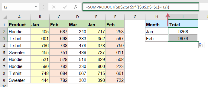

3.7.3 VLOOKUP and sum the first matched or all matched values with Kutools for Excel
Maybe the above formulas are difficult for you to remember, in this case, I will recommend a powerful feature - "Lookup and Sum" of "Kutools for Excel", with this feature, you can Vlookup and sum the first matching or all matching values in rows or columns as easily as possible.
- Click "Kutools" > "Super LOOKUP" > "LOOKUP and Sum" to enable this feature.
- Then specify the operations from the dialog box based on your need.

3.7.4 VLOOKUP and sum all matched values both in rows and columns
If you want to sum the values when you need to match both column and row, for example, to get the total value of the product Sweater in month Mar as below screenshot shown.
Here, you can use the SUMPRODCT function to accomplish this task.
Please apply the following formula into a cell, and then press "Enter" key to get the result, see screenshot:
=SUMPRODUCT(($B$2:$F$9)*($B$1:$F$1=I2)*($A$2:$A$9=H2))
Notes: In the above formula:
- "B2:F9" is the data range containing the numeric values that you want to sum;
- "B1:F1" is the column headers containing the lookup value that you want to sum based on;
- "I2" is the lookup value within the column headers you are looking for;
- "A2:A9" is the row headers containing the lookup value that you want to sum based on;
- "H2" is the lookup value within the row headers you are looking for.
3.8 VLOOKUP to merge two tables based on key columns
In your daily work, when analyzing data, you may need to gather all necessary information into a single table based on one or more key columns. To accomplish this task, you can use the INDEX and MATCH functions instead of the VLOOKUP function.
3.8.1 VLOOKUP to merge two tables based on one key column
For example, you have two tables, the first table containing the products and names data, and the second table contains the products and orders data, now, you want to combine these two tables by matching the common product column into one table.
Step 1: Apply the following formula
Please apply the following formula into a blank cell. Then, drag the fill handle down to the cells that you want to apply this formula
=INDEX($F$2:$F$8, MATCH($A2, $E$2:$E$8, 0))Result:
Now, you will get a merged table with the order column joining to the first table based on the key column data.
Notes: In the above formula:
- "A2" is the lookup value you are looking for;
- "F2:F8" is range of data that you want to return the matching values;
- "E2:E8" is lookup range which contains the lookup value.
3.8.2 VLOOKUP to merge two tables based on multiple key columns
If the two tables you want to join have multiple key columns, to merge the tables based on these common columns, please follow the steps below.
The generic formula is:
Notes:
- "lookup_table" is the data range contains the lookup data and matching records;
- "lookup_value1" is the first criteria you are looking for;
- "lookup_range1" is the data list contains the first criteria;
- "lookup_value2" is the second criteria you are looking for;
- "lookup_range2" is the data list contains the second criteria;
- "return_column_number" indicates the column number in the lookup_table that you want to return the matching value.
Step 1: Apply the following formula
Please apply the formula below into a blank cell where you want to put the result, and then press "Ctrl" + "Shift" + "Enter" keys together to get the first matched value, see screenshot:
=INDEX($E$2:$G$9, MATCH(1, ($A2=$E$2:$E$9) * ($B2=$F$2:$F$9), 0), 3)
Step 2: Fill the formula to other cells
Then, select the first formula cell, and drag the fill handle to copy this formula to other cells as you need:
3.9 VLOOKUP matching values across multiple worksheets
Have you ever needed to perform a VLOOKUP across multiple worksheets in Excel? For instance, if you have three worksheets with data ranges, and you want to retrieve specific values based on criteria from these sheets, you can follow the step-by-step tutorial VLOOKUP Values Across Multiple Worksheets to accomplish this task.

VLOOKUP matched values keep cell formatting
When looking up matched values, the original cell formatting such as font color, background color, data format, etc. will not be kept. To keep the cell or data formatting, this section will introduce some tricks for solving the jobs.
4.1 VLOOKUP matching value and keep cell color, font formatting
As we all known, the normal VLOOKUP function can only retrieve the matching value from another data range. However, there may be instances where you would like to get the corresponding value along with the cell formatting, such as the fill color, font color, and font style. In this section, we will discuss how to retrieve matching values while preserving source formatting in Excel.
Please do with the following steps to lookup and return its corresponding value along with cell formatting:
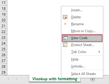
Step 1: Copy the code 1 into the Sheet Code Module
- In the worksheet contains the data you want to VLOOKUP, right click the sheet tab and select "View Code" from the context menu. See screenshot:
- In the opened "Microsoft Visual Basic for Applications" window, please copy the below VBA code into the Code window.
- VBA code 1: VLOOKUP to get cell formatting along with lookup value
-
Sub Worksheet_Change(ByVal Target As Range) 'Updateby Extendoffice Dim I As Long Dim xKeys As Long Dim xDicStr As String On Error Resume Next Application.ScreenUpdating = False xKeys = UBound(xDic.Keys) If xKeys >= 0 Then For I = 0 To UBound(xDic.Keys) xDicStr = xDic.Items(I) If xDicStr <> "" Then Range(xDic.Keys(I)).Interior.Color = _ Range(xDic.Items(I)).Interior.Color Range(xDic.Keys(I)).Font.FontStyle = _ Range(xDic.Items(I)).Font.FontStyle Range(xDic.Keys(I)).Font.Size = _ Range(xDic.Items(I)).Font.Size Range(xDic.Keys(I)).Font.Color = _ Range(xDic.Items(I)).Font.Color Range(xDic.Keys(I)).Font.Name = _ Range(xDic.Items(I)).Font.Name Range(xDic.Keys(I)).Font.Underline = _ Range(xDic.Items(I)).Font.Underline Else Range(xDic.Keys(I)).Interior.Color = xlNone End If Next Set xDic = Nothing End If Application.ScreenUpdating = True End Sub 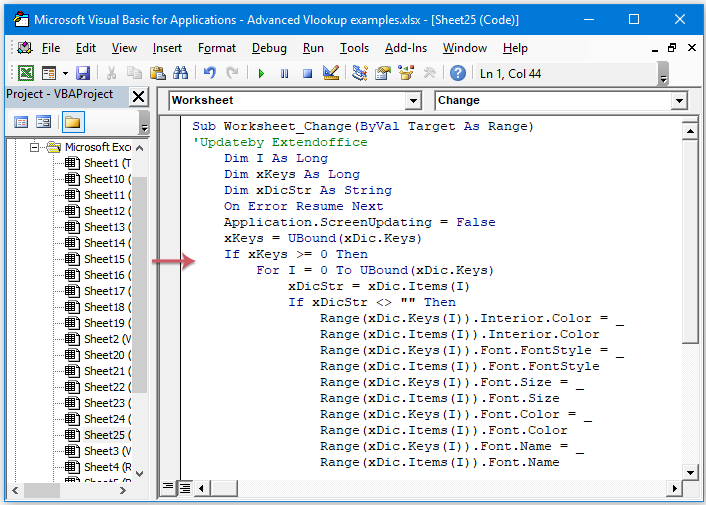


Step 2: Copy the code 2 into the Module window
- Still in the "Microsoft Visual Basic for Applications" window, click "Insert" > "Module", and then copy the below VBA code 2 into the "Module" window.
- VBA code 2: VLOOKUP to get cell formatting along with lookup value
-
Public xDic As New Dictionary Function LookupKeepFormat (ByRef FndValue, ByRef LookupRng As Range, ByRef xCol As Long) Dim xFindCell As Range On Error Resume Next Set xFindCell = LookupRng.Find(FndValue, , xlValues, xlWhole) If xFindCell Is Nothing Then LookupKeepFormat = "" xDic.Add Application.Caller.Address, "" Else LookupKeepFormat = xFindCell.Offset(0, xCol - 1).Value xDic.Add Application.Caller.Address, xFindCell.Offset(0, xCol - 1).Address End If End Function 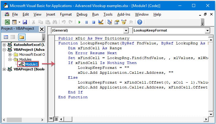

Step 3: Select the option for VBAproject
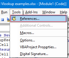
- After inserting the above codes, then click "Tools" > "References" in the "Microsoft Visual Basic for Applications" window. Then check the "Microsoft Scripting Runtime" checkbox in the "References – VBAProject" dialog box. See screenshots:

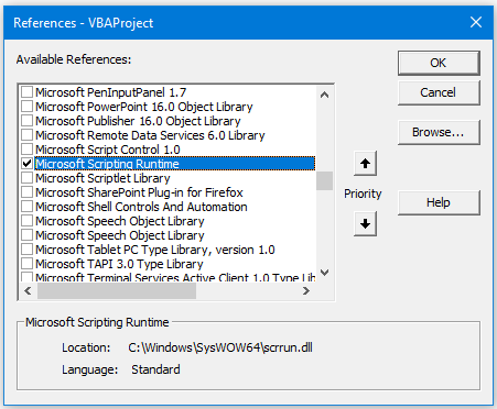
- Then, click "OK" to close the dialog box, and then save and close the code window.


Step 4: Type the formula for getting the result
- Now, go back to the worksheet, apply the following formula. And then, drag the fill handle down to get all results along with their formatting. See screenshot:
=LookupKeepFormat(E2,$A$1:$C$10,3)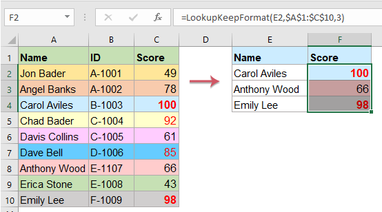

Notes: in the above formula:
- "E2" is the value you will look up;
- "A1:C10" is the table range;
- "3" is the column number of the table from which you want to retrieve the matched value.
4.2 Keep the date format from a VLOOKUP returned value
When using the VLOOKUP function to lookup and return a value with date format, the returned result may display as a number. To keep the date format in the returned result, you should enclose the VLOOKUP function within the TEXT function.
Step 1: Apply the following formula
Please apply the formula below into a blank cell. Then, drag the fill handle to copy this formula to other cells.
=TEXT(VLOOKUP(E2,$A$2:$C$9,3,FALSE),"mm/dd/yyyy")Result:
All the matched dates have been returned as below screenshot shown:
Notes: In the above formula:
- "E2" is the lookup value;
- "A2:C9" is the lookup range;
- "3" is the column number you want the value returned;
- "FALSE" indicates to get an exact match;
- "mm/dd/yyyy" is the date format you want to keep.
4.3 Return cell comment from VLOOKUP
Have you ever needed to retrieve both the matching cell data and its associated comment using VLOOKUP in Excel, as shown in the following screenshot? If so, the User Defined Function provided below can help you accomplish this task.
Step 1: Copy the code into a Module
- Hold down the "ALT" + "F11" keys to open the "Microsoft Visual Basic for Applications" window.
- Click "Insert" > "Module", then copy and paste the following code in the "Module" window.
VBA code: Vlookup and return matching value with cell comment:Function VlookupComment(LookVal As Variant, FTable As Range, FColumn As Long, FType As Long) As Variant 'Updateby Extendoffice Application.Volatile Dim xRet As Variant 'could be an error Dim xCell As Range xRet = Application.Match(LookVal, FTable.Columns(1), FType) If IsError(xRet) Then VlookupComment = "Not Found" Else Set xCell = FTable.Columns(FColumn).Cells(1)(xRet) VlookupComment = xCell.Value With Application.Caller If Not .Comment Is Nothing Then .Comment.Delete End If If Not xCell.Comment Is Nothing Then .AddComment xCell.Comment.Text End If End With End If End Function - Then save and close the code window.
Step 2: Type the formula to get the result
- Now, enter the following formula, and drag the fill handle to copy this formula to other cells. It will return both the matched values and comments simultaneously, see screenshot:
=vlookupcomment(D2,$A$2:$B$9,2,FALSE)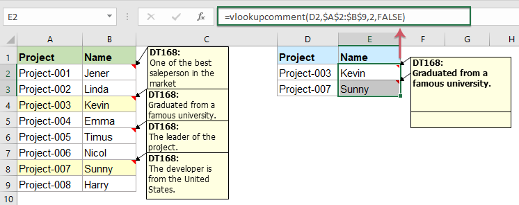

Notes: In the above formula:
- "D2" is the lookup value you want to return its corresponding value;
- "A2:B9" is the data table you want to use;
- "2" is the column number which contains the matched value you want to return;
- "FALSE" indicates to get an exact match.
4.4 VLOOKUP numbers stored as text
For instance, I have a range of data where the ID number in the original table is in number format and the ID number in the lookup cells is stored as text, you may encounter an #N/A error when using the normal VLOOKUP function. In this case, to retrieve the correct information, you can wrap the TEXT and VALUE functions within the VLOOKUP function.Below is the formula to achieve this: 
Step 1: Apply and fill the following formula
Please apply the following formula into a blank cell, and then drag the fill handle down to copy this formula.
=IFERROR(VLOOKUP(VALUE(D2),$A$2:$B$8,2,0),VLOOKUP(TEXT(D2,0),$A$2:$B$8,2,0))Result:
Now, you will get the correct results as below screenshot shown:
Notes:
- In the above formula:
- "D2" is the lookup value you want to return its corresponding value;
- "A2:B8" is the data table you want to use;
- "2" is the column number which contains the matched value you want to return;
- "0" indicates to get an exact match.
- This formula also works well if you are not sure where you have numbers and where you have text.
Best Office Productivity Tools
Supercharge Your Excel Skills with Kutools for Excel, and Experience Efficiency Like Never Before. Kutools for Excel Offers Over 300 Advanced Features to Boost Productivity and Save Time. Click Here to Get The Feature You Need The Most...
Office Tab Brings Tabbed interface to Office, and Make Your Work Much Easier
- Enable tabbed editing and reading in Word, Excel, PowerPoint, Publisher, Access, Visio and Project.
- Open and create multiple documents in new tabs of the same window, rather than in new windows.
- Increases your productivity by 50%, and reduces hundreds of mouse clicks for you every day!
All Kutools add-ins. One installer
Kutools for Office suite bundles add-ins for Excel, Word, Outlook & PowerPoint plus Office Tab Pro, which is ideal for teams working across Office apps.
- All-in-one suite — Excel, Word, Outlook & PowerPoint add-ins + Office Tab Pro
- One installer, one license — set up in minutes (MSI-ready)
- Works better together — streamlined productivity across Office apps
- 30-day full-featured trial — no registration, no credit card
- Best value — save vs buying individual add-in
Table of contents
- 1. Introduction of VLOOKUP function
- 2. Basic VLOOKUP examples
- 2.1 Exact and approximate Vlookup
- Exact match
- Approximate match
- 2.2 Case sensitive Vlookup
- 2.3 Vlookup from right to left
- 2.4 Vlookup the second, nth or last matching value
- The second or nth matching value
- The last matching value
- 2.5 Vlookup between two values
- By using formula
- By using a handy feature - Kutools
- 2.6 Partial match Vlookup
- 2.7 Vlookup from another worksheet
- 2.8 Vlookup from another workbook
- 2.9 Fix 0 or #N/A error value in Vlookup
- 3. Advanced VLOOKUP examples
- 3.1 Two-way lookup
- 3.2 Vlookup based on more criteria
- By using formulas
- By using a smart feature - Kutools
- 3.3 Vlookup multiple matching values
- Return values horizontally
- Return values vertically
- Return values into one cell
- 3.4 Vlookup entire row
- 3.5 Nested Vlookup
- 3.6 Check if value exists
- 3.7 Vlookup and sum
- In rows
- In columns
- With a powerful feature - Kutools
- Both in rows and columns
- 3.8 Vlookup to merge two tables
- By one key column
- By multiple key columns
- 3.9 Vlookup across multiple worksheets
- 4. VLOOKUP and keep cell formatting
- 4.1 Keep color and font formatting
- 4.2 Keep the date format
- 4.3 Keep cell comment
- 4.4 Numbers stored as text
- The Best Office Productivity Tools