How to flip / reverse a column of data order vertically in Excel?
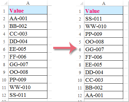
Sometimes, you may want to flip a column of data order vertically in Excel as the left screenshot shown. It seems quite hard to reverse the data order manually, especially for a lot of data in the column. This article will guide you to flip or reverse a column data order vertically quickly.
Flip a column of data order in Excel with Sort command
Flip a column of data order in Excel with VBA
Several clicks to flip a column of data order with Kutools for Excel
Flip a column of data order in Excel with Sort command
Using Sort command can help you flip a column of data in Excel with following steps:
1. Insert a series of sequence numbers besides the column. In this case, in insert 1, 2, 3…, 7 in Column B, then select B2:B12, see screenshot:

2. Click the Data > Sort Z to A, see screenshot:

3. In the Sort Warning dialog box, check the Expand the selection option, and click the Sort button.

4. Then you will see the number order of Column A is flipped. And you can delete or hide the Column B according to your needs. See the following screenshot:

This method is also applied to reversing multiple columns of data order.
Easily flip a column of date vertically with several clicks:
TheFlip Vertical Range utility of Kutools for Excel can help you quickly flip a column of date vertically with only several clicks. You just need to select the range and enable the function to acheive it. Download Kutools for Excel Now! (30-day free trail)

Flip a column of data order in Excel with VBA
If you know how to use a VBA code in Excel, you may flip / reverse data order vertically as follows:
1. Hold down the Alt + F11 keys in Excel, and it opens the Microsoft Visual Basic for Applications window.
2. Click Insert > Module, and paste the following macro in the Module Window.
VBA: Flip / reverse a range data order vertically in Excel.
Sub FlipColumns()
'Updateby20131126
Dim Rng As Range
Dim WorkRng As Range
Dim Arr As Variant
Dim i As Integer, j As Integer, k As Integer
On Error Resume Next
xTitleId = "KutoolsforExcel"
Set WorkRng = Application.Selection
Set WorkRng = Application.InputBox("Range", xTitleId, WorkRng.Address, Type:=8)
Arr = WorkRng.Formula
For j = 1 To UBound(Arr, 2)
    k = UBound(Arr, 1)
    For i = 1 To UBound(Arr, 1) / 2
        xTemp = Arr(i, j)
        Arr(i, j) = Arr(k, j)
        Arr(k, j) = xTemp
        k = k - 1
    Next
Next
WorkRng.Formula = Arr
End Sub
3. Press the F5 key to run this macro, a dialog is popped up for you to select a range to flip vertically, see screenshot:

4. Click OK in the dialog, the range is flipped vertically, see screenshot:
Several clicks to flip a column of data order with Kutools for Excel
If you have Kutools for Excel installed, you can reverse the numbers order of columns with Flip Vertical Range tool quickly.
1. Select the column of date you will flip vertically, then click Kutools > Range > Flip Vertical Range > All / Only flip values. See screenshot:

Note: If you want to flip vaues along with cell formatting, plesae select the All option. For only flipping values, please select the Only flip values option.
Then the selected data in the column has been flipped vertically. See screenshot:
Tip: If you also need to flip data horizontally in Excel. Please try the Flip Horizontal Range utility of Kutools for Excel. You just need to select two ranges firstly, and then apply the utility to acheive it as below screenshot shown.

Then the selected ranges are flipped horizontally immediately.

If you want to have a free trial (30-day) of this utility, please click to download it, and then go to apply the operation according above steps.
Related article:
How to flip / reverse a row of data order in Excel quickly?
Best Office Productivity Tools
Supercharge Your Excel Skills with Kutools for Excel, and Experience Efficiency Like Never Before. Kutools for Excel Offers Over 300 Advanced Features to Boost Productivity and Save Time. Click Here to Get The Feature You Need The Most...
Office Tab Brings Tabbed interface to Office, and Make Your Work Much Easier
- Enable tabbed editing and reading in Word, Excel, PowerPoint, Publisher, Access, Visio and Project.
- Open and create multiple documents in new tabs of the same window, rather than in new windows.
- Increases your productivity by 50%, and reduces hundreds of mouse clicks for you every day!
All Kutools add-ins. One installer
Kutools for Office suite bundles add-ins for Excel, Word, Outlook & PowerPoint plus Office Tab Pro, which is ideal for teams working across Office apps.
- All-in-one suite — Excel, Word, Outlook & PowerPoint add-ins + Office Tab Pro
- One installer, one license — set up in minutes (MSI-ready)
- Works better together — streamlined productivity across Office apps
- 30-day full-featured trial — no registration, no credit card
- Best value — save vs buying individual add-in