How to highlight cell if value is greater than another cell in Excel?
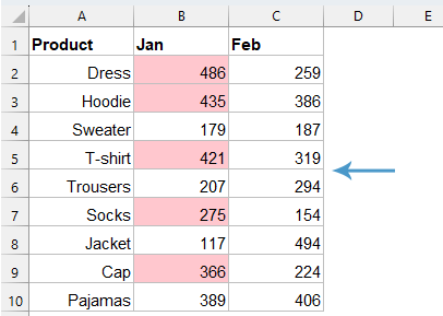
To compare values in two columns - for example, if a value in column B is greater than the corresponding value in column C in the same row - you can highlight the values in column B, as shown in the left screenshot. This article introduces several methods to highlight cells where one value is greater than another in Excel.
Highlight cell if value is greater than another cell by using Conditional Formatting
Highlight cell if value is greater than another cell by using Kutools AI Aide
Highlight cell if value is greater than another cell by using Conditional Formatting
To highlight the cells whose values are greater than the values in another column in the same row, the Conditional Formatting in Excel can do you a favor.
1. Select the data list that you want to highlight, and then click "Home" > "Conditional Formatting" > "New Rule", see screenshot:

2. In the opened "New Formatting Rule" dialog box:
- Click "Use a formula to determine which cells to format" from the" Select a Rule Type" list box;
- Type this formula: =B2>C2 into the "Format values where this formula is true" textbox;
- And then, click" Format" button.

3. In the popped-out "Format Cells" dialog, under the "Fill" tab, choose one color you like to highlight the greater values with, see screenshot:

4. Then, click "OK" > "OK" to close the dialog boxes. Now, you can see the values in column B greater than the values in column C based on the row are highlighted at once, see screenshot:


And you will get the result as below screenshot shown:

Highlight cell if value is greater than another cell by using Kutools AI Aide
Tired of searching for differences in your data? With Kutools AI Aide, it's a breeze! Just pick your numbers, tell us which one you're comparing against, and voilà! We'll make the differences pop out, whether it's sales, project goals, or anything else. Spend less time hunting for changes and more time making smart decisions.
After installing Kutools for Excel, please click "Kutools AI" > "AI Aide" to open the "Kutools AI Aide" pane:
- Type your requirement into the chat box, and then click "Send" button or press Enter key to send the question;
- After analyzing, click "Execute" button to run. Kutools AI Aide will process your request using AI and return the results directly in Excel.

More relative articles:
- Color Alternate Rows For Merged Cells
- It is very helpful to format alternate rows with a different color in a large data for us to scan the data, but, sometimes, there may be some merged cells in your data. To highlight the rows alternately with a different color for the merged cells as below screenshot shown, how could you solve this problem in Excel?
- Highlight Largest / Lowest Value In Each Row Or Column
- If you have multiple columns and rows data, how could you highlight the largest or lowest value in each row or column? It will be tedious if you identify the values one by one in each row or column. In this case, the Conditional Formatting feature in Excel can do you a favor. Please read more to know the details.
- Highlight Approximate Match Lookup
- In Excel, we can use the Vlookup function to get the approximate matched value quickly and easily. But, have you ever tried to get the approximate match based on row and column data and highlight the approximate match from the original data range as below screenshot shown? This article will talk about how to solve this task in Excel.
- Highlight Entire / Whole Row While Scrolling
- If you have a large worksheet with multiple columns, it will be difficult for you to distinguish data on that row. In this case, you can highlight the whole row of active cell so that you can quickly and easily view the data in that row when you scroll down the horizontal scroll bar .This article, I will talk about some tricks for you to solve this problem.
Best Office Productivity Tools
Supercharge Your Excel Skills with Kutools for Excel, and Experience Efficiency Like Never Before. Kutools for Excel Offers Over 300 Advanced Features to Boost Productivity and Save Time. Click Here to Get The Feature You Need The Most...
Office Tab Brings Tabbed interface to Office, and Make Your Work Much Easier
- Enable tabbed editing and reading in Word, Excel, PowerPoint, Publisher, Access, Visio and Project.
- Open and create multiple documents in new tabs of the same window, rather than in new windows.
- Increases your productivity by 50%, and reduces hundreds of mouse clicks for you every day!
All Kutools add-ins. One installer
Kutools for Office suite bundles add-ins for Excel, Word, Outlook & PowerPoint plus Office Tab Pro, which is ideal for teams working across Office apps.
- All-in-one suite — Excel, Word, Outlook & PowerPoint add-ins + Office Tab Pro
- One installer, one license — set up in minutes (MSI-ready)
- Works better together — streamlined productivity across Office apps
- 30-day full-featured trial — no registration, no credit card
- Best value — save vs buying individual add-in