How to connect a single slicer to multiple pivot tables in Excel?
By default, an Excel pivot table slicer is only connected to the pivot table that you are inserting the slicer from. In some cases, to make pivot tables work more efficiently, you may need to use a single slicer to control more than one pivot table in your workbook. This tutorial provides two methods for you to connect a single slicer to multiple pivot tables, not only from the same data set, but from different data sets.
Connect a single slicer to multiple pivot tables from the same data set
Connect a single slicer to multiple pivot tables from different data sets
Connect a single slicer to multiple pivot tables from the same data set
As shown in the screenshot below, there is a sales table in the range A1:H20, now, you want to create two pivot tables to analyze the data, and then use a single slicer to control these two pivot tables. Please do as follows to get it done.

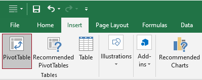
1. First, you need to create two pivot tables based on the table range.
2. In the opening Create PivotTable dialog box, specify where to place the pivot table in the Choose where you want the PivotTable report to be placed section, and then click the OK button.

3. Now you need to add fields to your pivot table. Please drag the needed fields to the target areas one by one.
In this case, I drag the Date field from the field list to the Rows area and drag the Sales field to the Values area. See screenshot:

4. Go ahead to insert the second pivot table for the table range.
Here I created two pivot tables as shown in the screenshot below.

5. Now you need to insert a slicer (this slicer will be used to control both pivot tables). Click on any cell in one pivot table, such as PivotTable1, and then go to click Analyze (under the PivotTable Tools tab) > Insert Slicer.

6. In the opening Insert Slicers dialog box, tick the column you want to use to filter both the two pivot tables, and then click OK.

7. Then a slicer is inserted into the current worksheet. Since the slicer is now only connected to the PivotTable1, you need to link it to the PivotTable2 as well. Right click the slicer and click Report Connections from the context menu.

8. In the Report Connections dialog box, check the pivot tables that you need to connect to this slicer at the same time, and then, click the OK button.

Now the slicer is connected to both the pivot tables.

Unlock Excel Magic with Kutools AI
- Smart Execution: Perform cell operations, analyze data, and create charts—all driven by simple commands.
- Custom Formulas: Generate tailored formulas to streamline your workflows.
- VBA Coding: Write and implement VBA code effortlessly.
- Formula Interpretation: Understand complex formulas with ease.
- Text Translation: Break language barriers within your spreadsheets.
Connect a single slicer to multiple pivot tables from different data sets
The above pivot tables all come from the same data set. If the pivot tables come from different data sets, you need to handle this task in a different way.
As shown in the screenshot below, supposing you have two worksheets (August and September) containing monthly sales for different months, and the data in these two tables needs to be analyzed by different pivot tables. Also, you need a single slicer to control both the pivot tables. The method in this section can do you a favor.
Note: Both worksheets should have the same column data that used to create the slicer.


Create tables
1. Make sure both the data ranges are in Table format. If not, you need to convert them to Tables.

Rename tables
2. After converting the ranges to tables, please rename the tables with descriptive names. Here I change the table names to match the names of the worksheets, i.e. August and September.
Click on any cell in the table, go to the Design tab, and then modify the table name in the Table Name text box.

Create a helper column for creating the slicer and convert to table
3. Create a new worksheet by clicking the New sheet button and rename the newly created worksheet as you need.

4. Go back to any worksheet containing data, such as “August”, select the column data that you want to use to create the slicer. Here I select the Product column in the worksheet “August”. Press Ctrl + C keys to copy the data, then press the Ctrl + V keys to paste the data in the newly created worksheet.
5. Keep the data selected in the newly created worksheet, click Data > Remove Duplicates.

6. In the Remove Duplicates dialog box, click the OK button.

7. Then a dialog box pops up to tell you how many duplicates are removed from the list, click OK to close the dialog box.
8. After removing duplicates, select the remained data cells and press the Ctrl + T keys. In the popping up Create Table dialog box, check the My table has headers box and then click OK.

9. Change the table name in this newly created worksheet to match the column header, which is “Product”.
Create pivot tables from different data sets
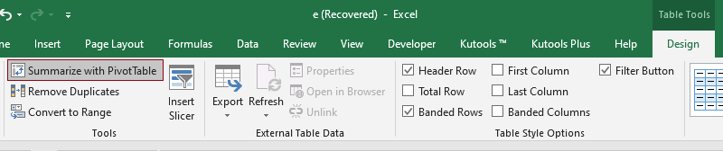
10. Go back to the worksheet named “August”, click on any cell in the table and go to click Design > Summarize with PivotTable.
11. In the create PivotTable dialog box, you need to configure as follows.

12. Now you need to add fields to your pivot table. Please drag the needed fields to the target areas one by one.
In this case, I drag the Date field from the field list to the Rows area and drag the Sales field to the Values area. See screenshot:

13. Go to the worksheet named “September”, click on any cell in the table and go to click Design > Summarize with PivotTable.
14. Then you need to configure the settings in the Create PivotTable dialog box.
The different setting here is that you need to select the Existing Worksheet option and select a cell in the worksheet where the first pivot table is placed.

15. Now add fields to this pivot table.

Now you get two pivot tables from different data sets placed in one worksheet.

Insert a pivot table slicer
16. Click on any pivot table (here I click on any cell in the first pivot table), click Analyze > Insert Slicer.

17. In the Insert Slicers dialog box, you need to configure as follows.

Build the relationships between the existing tables
18. Now you need to build the relationship between the existing tables. Click on any pivot table, and then click Analyze > Relationships.

19. In the opening Manage Relationships dialog box, click the New button.

20. In the Create Relationship dialog box, you need to build the first relationships as follows.

21. Then it returns to the Manage Relationships dialog box, click the New button again.

22. In the Create Relationship dialog box, you need to build the second relationships as follows.

23. When it returns to the Manage Relationships dialog box, you can see the two relationships listed inside. Click the Close button to close the dialog box.
24. Right click the slicer and click Report Connections from the context menu.

25. In the Report Connections dialog box, check the pivot table that you also need it to connect to this slicer and click the OK button.

Now you have finished all steps.
The slicer is now connected to both the pivot tables from different data sets.
Best Office Productivity Tools
Supercharge Your Excel Skills with Kutools for Excel, and Experience Efficiency Like Never Before. Kutools for Excel Offers Over 300 Advanced Features to Boost Productivity and Save Time. Click Here to Get The Feature You Need The Most...
Office Tab Brings Tabbed interface to Office, and Make Your Work Much Easier
- Enable tabbed editing and reading in Word, Excel, PowerPoint, Publisher, Access, Visio and Project.
- Open and create multiple documents in new tabs of the same window, rather than in new windows.
- Increases your productivity by 50%, and reduces hundreds of mouse clicks for you every day!
All Kutools add-ins. One installer
Kutools for Office suite bundles add-ins for Excel, Word, Outlook & PowerPoint plus Office Tab Pro, which is ideal for teams working across Office apps.
- All-in-one suite — Excel, Word, Outlook & PowerPoint add-ins + Office Tab Pro
- One installer, one license — set up in minutes (MSI-ready)
- Works better together — streamlined productivity across Office apps
- 30-day full-featured trial — no registration, no credit card
- Best value — save vs buying individual add-in